Exploration of Wireless Multimedia Sensor Network
Based on Joint Photographic Experts Group Image
Coding Algorithm
https://doi.org/10.3991/ ijoe.v15i01.9781Jie He
ChongQing Technology and Business Institute, ChongQing, China
Abstract—To study the performance of image coding and image transmission of wireless video sensor node in wireless multimedia sensor network, the challenges and design objectives of image coding technology in wireless multimedia sensor network are discussed, and the classification and exploration are carried out from two aspects: individual source coding and distributed source coding. The compression of video monitoring image sequence in wireless multimedia sensor network is studied and a low complexity image coding scheme based on change detection and improved Joint Photographic Experts Group (JPEG) algorithm is proposed. The moving target in the monitoring image is located with the change detection algorithm, that is, the area of interest. Only the region of interest is transmitted to reduce the quantity of data transmission and adapt to the limited storage and forwarding capability of wireless sensor nodes; The Discrete Cosine Transform (DCT) and quantization processes in Joint Photographic Experts Group (JPEG) algorithm are improved to reduce the computational complexity and adapt to the limited computing power of wireless sensor nodes. The analysis of algorithm complexity and the results of simulation experiment show that the proposed method can effectively reduce the data communication amount of wireless sensor nodes and the energy consumption in the calculation process while ensuring the image quality required by the application. Wireless multimedia sensor network is a new and interdisciplinary subject. The study of it is also multidirectional and multi-angle. The image coding algorithm of wireless multimedia sensor network is studied deeply. Although some achievements have been made, there are still a lot of problems that need to be further studied.
Keywords—Wireless multimedia, sensor networks, image coding, Joint Photographic Experts Group (JPEG)
1
Introduction
data are analyzed by the operator. With the development of image sensor technology, low-power image sensors have emerged in many products such as mobile phones, toys, computers and robots [1]. In addition, the development of sensor networks and distributed processing technologies have facilitated the use of image sensors in these networks, resulting in the emergence of multimedia sensor networks. The combination of low-power wireless networking technology and inexpensive cameras and microphones has led to the creation of distributed networked systems, that is, the wireless multimedia sensor network system [2]. The wireless multimedia sensor network is a new type of sensor network, which includes a camera, a microphone, and other sensor nodes that can generate multimedia data, and requires quantitative multimedia management. A large number of video nodes in wireless multimedia sensor networks form a distributed system. Video nodes can process image data locally and extract relevant information. It can cooperate with other video nodes to complete some specific application tasks, and it can provide system users with a rich description of the captured events.
2
Literature Review
Costa et al. (2015) believe that the design goal in the field of wireless multimedia sensor network coding is to find a coding method with low complexity, low output bandwidth, fault tolerance and as little power consumption as possible. At present, image encoding algorithms in wireless multimedia sensor networks mainly include two types: independent source coding and distributed source coding [3].
Khan et al. (2017) believe that independent source coding means that the coding information of each node is independent of other nodes. In multimedia coding, independent source coding is relatively simple and there is no kind of interaction between nodes. However, there is a great deal of coverage and coincidence of multimedia sensors for specific events. The compression of independent source codes produces a lot of redundancy. Because all sensor nodes are trying to maintain the best quality of the transmitted image, much of the same data is transmitted to the sink or base station, resulting in a large number of copies of the same data. These copies may lead to network traffic congestion and energy exhaustion. Therefore, there is still much room for the improvement of independent source coding [4].
Usman et al. (2018) believe that distributed source code is compressed on multiple relevant sensors and decoded by the central decoder at the base station or sink node. Distributed source coding changes the traditional one-to-many image coding mode used in most image encoder and decoders. In one-to-many coding modes, the encoder requires complex coding, and the decoder part is relatively simple. However, distributed source coding uses a many-to-one coding mode, changing from a complex encoder to a complex decoder. Therefore, the encoder at the image sensor node can be simplified, requiring only less resources, and a more complex decoder is set up at the sink node or the base station [5].
and JPEG2000-based coding. Although the JPEG2000-based coding can support the coding of interest regions, in the case of image compression of natural scenes, when the compression rate is relatively large, the quality of the images restored by this method is high. However, JPEG2000 uses a compression algorithm based on wavelet transform. Wavelet transform has the problems of high computational complexity and large storage capacity. In order to apply the wavelet transform-based compression algorithm to the wireless multimedia sensor network, the problem that needs to be solved is to reduce the computational complexity and the memory requirement [6].
Ghadi et al. (2016) believe that for the JPEG-based coding, the industry has studied some methods for locating interest areas and improving JPEG compression for DCT transforms. The coding combined with the region of interest can significantly reduce the amount of data that needs to be transmitted, the simplification of the DCT transform can reduce the computational complexity. However, these methods also have some drawbacks and limitations: no selection method for the region of interest is given, the default region of interest is used for encoding, and the algorithm lacks portability; without energy analysis, the energy consumption of the entire process occurs in the coding and communication parts, without considering the overall energy consumption [7].
3
JPEG image coding algorithm optimization
3.1 Change detection algorithm
The change detection algorithm is used to detect the change area in the image sequence captured at different times in the same scene. The active block is found by comparing the current frame with the reference frame, thereby obtaining a connected area related to the moving object [8]. The goal of video surveillance is to detect and track the targets that enter the surveillance area. According to different application scenarios, the user's focus is also different [9]. The change detection algorithm can locate possible targets in the image, and the areas containing these targets are potential areas of interest [10]. The first step in determining the area of interest is to locate the area of change, mark the area of change, and then perform in-depth processing to track and identify the target.
. (1) Among them, C((i-1)*8+k,(j-1)*8+l) is the pixel value of a pixel belonging to the set A in one DCT block in the current frame. R((i−1)*8+k,(j−1)*8+l) is the pixel value of a pixel belonging to the set A in one DCT block in the reference frame. (i,j) represents the position of the DCT block in one frame of image, and 1≤i≤[m/8] and 1≤j≤[n/8] indicate the size of the image.
Pixel scan mode 1
Fig. 1. Pixel scan mode 2
Calculate the sum of the absolute differences of the pixels belonging to the set A in all DCT blocks in the current frame and the reference frame. If the sum of the absolute difference of a DCT block is greater than zero, the DCT block is considered to have changed, otherwise it is considered that the block has not changed. Other external causes such as noise may also cause changes in the DCT block, such as camera movement, sensor noise, light source changes, atmospheric changes, etc. By selecting an appropriate threshold for segmentation, the changes caused by the target motion can be distinguished from those caused by other causes. In spite of it, change detection can’t distinguish the shadows and reflections of moving objects, but they are all considered as change areas. For a resource-constrained WMSN, the rough edges of the target are more energy-efficient than the fine edges. Therefore, only one threshold
|
l)
8
*
1)
-(j
k,
8
*
1)
-R((i
)
8
*
)
1
(
,
8
*
)
1
((
|
)
,
(
81 8
1
+
+
+
-+
-=
åå
= =
k l
l
j
k
i
C
j
is selected to distinguish between noise-induced changes and changes caused by moving targets. By comparing with the reference frame, the DCT block in the image is divided into three types: stationary, noise, and motion, judgment criteria are as follows:
If (SAD = 0), the block is marked as stationary; If (0<SAD<TH), the block is marked as noise; If (TH<SAD), the block is marked as moving.
Whether change detection can distinguish between noise and moving targets, the choice of threshold is critical. The choice of threshold depends on the scene and the degree of possible camera movement, as well as observation conditions (such as lighting) that change over time. In general, it is obviously more reasonable to select the segmentation threshold according to the image content, but the threshold used here depends on experience.
3.2 Threshold selection algorithm
The grayscale difference image d(k)=y1(k)-y2(k), D={d(k)}, y1(k) and y2(k) are the grayscale values of the two images at position k. The change mask consists of a binary label q(k). When the pixel point has no change or the change is caused by noise, q(k)=u; when the pixel point changes, q(k)=c. When the difference image is given, the posterior probability of the change mask is Pr(Q|D).
Assuming that the label value q(K) of only pixel i in an image is not determined, the estimated change mask Q becomes q(i)=u or q(i)=c. The change mask obtained from q(i)=u is Qiu and the change mask obtained from q(i)=c is Qic, the criterion is as follows (2).
. (2)
t is a threshold. When q(i)=u, the value on the left is greater than t, and when q(i)=c, the value on the left is less than t. According to the Bayesian formula, this criterion can be written as (3).
. (3)
p(D|Q) represents the conditional probability of the difference image D when given a change mask Q, which is also a probability function of Q. Pr(Qiu) and Pr(Qic) are the prior probabilities of Qiu and Qic.
t
D
Q
D
Q
c
i
t
D
Q
D
Q
u
i
i c i u i c iu
>
=
>
Assuming that the gray difference is conditionally independent, then p(D|Q) = Πkp(d(k)|q(k)) can be obtained, the above decision criterion can be simplified as (4).
. (4)
p(d(i)|Hj) represents the probability that the hypothesis Hj,j=0,1 for the pixel i. In order to make the detection more reliable, it can’t be judged merely by the gray difference d(i) of the pixel i, but some local gray difference samples di should be selected. The sample consists of the pixel gray difference d(k) in the sliding window wi centered on the pixel i. Using these samples for testing, the judgment formula can be expressed as (5).
. (5)
In contrast to the above formula, this criterion is based on the entire sample space di={d(k)|k∈Wi}. In order to convert the above equation into a practical decision criterion, it must be assumed for the conditional density p(d(k)|Hj), j=0,1, and the prior probability. Starting from p(d(k)|Hj), it is assumed that the gray value difference follows a zero mean Gaussian distribution, and the variances for H0 and H1 are σ20 and σ21, respectively. Because the difference in the change area is usually very large, the variance σ21 is much larger than the noise-induced variance σ20, and the estimation range is σ21>100σ20. The above criteria can be expressed as (6).
. (6)
Where is the sum of squares of gray difference value d(k) in normalized
window Wi, i.e., . Nw represents the size of the window wi in the
image.
)
Pr(
)
Pr(
)
|
)
(
(
)
|
)
(
(
,
c
)
(
q
)
Pr(
)
Pr(
)
|
)
(
(
)
|
)
(
(
,
)
(
q
1 0 1 0 i u i c i u i cQ
Q
t
H
i
d
p
H
i
d
p
i
Q
Q
t
H
i
d
p
H
i
d
p
u
i
>
=
>
=
)
Pr(
)
Pr(
)
|
(
)
|
(
,
)
(
q
)
Pr(
)
Pr(
)
|
(
)
|
(
,
)
(
q
1 0 1 0 i u i c i i i u i c i iQ
Q
t
H
d
p
H
d
p
c
i
Q
Q
t
H
d
p
H
d
p
u
i
>
=
>
=
)
Pr(
)
Pr(
)
(
)
1
(
2
1
exp
,
)
(
q
)
Pr(
)
Pr(
)
(
)
1
(
2
1
exp
,
)
(
q
1 0 2 2 1 2 0 1 0 2 2 1 2 0 i u i c Nw i i u i c Nw iQ
Q
t
c
i
Q
Q
t
u
i
s
s
s
s
s
s
s
s
>
þ
ý
ü
î
í
ì
D
-=
>
þ
ý
ü
î
í
ì
D
-=
2 iD
å
Î=
D
i w kk
d
(
)
1
22 0 2
3.3 Motion detection of light changes
After the target image is determined, a difference or ratio image is generated, and then a threshold is used to divide the pixels into two categories: motion or no motion. Many histogram-based thresholding methods binarize pixels in the histogram with two major peaks and valleys between them. One or more Gaussian functions or other functions are used by these documents to estimate the distribution of brightness. In this case, other shape parameters of the center and the function need to be located and decided. The center and shape parameters are combined to build approximate functions, but they also interfere with each other during the fast convergence to the appropriate solution. Therefore, a simple and more flexible threshold-based approach is quite necessary. A method of using a cumulative histogram inflection point detection to determine the image threshold is presented in this section.
Many scholars have studied the problem of image processing and motion analysis with changes in light over time. According to a simplified image formation model, the image is the result of the human representation of the light reflected by the object in the observation scene. In fact, this simple model assumes that the combined effect of several light sources is a unified lighting source for a scene. Based on this assumption, it can be considered that the brightness detected by the sensor is generated by the reflection of light and the image surface projected onto the sensor. If f (x, y) represents the brightness of the sensor at the corresponding position (x, y), r (x, y) represents the reflection coefficient of the object surface projected onto the sensor, i(x,y) represents the light received by the surface of the object, then f(x,y)=i(x,y)r(x,y) can be obtained.
In the other case, when the luminance distribution is similar but the motion occurs in a part of the pixels, the ratio of the pixels without motion is 1 and the moving pixels have prominent ratios in the ratio map. Therefore, motion can be easily detected based on the ratio map. In this case, for the difference image, the pixel value without motion is 0, and the moving pixel has a significant difference. It can be concluded that the ratio map is more effective for motion detection than the difference map when considering the change of illumination.
The difference map and ratio map between two grayscale images can be obtained by subtracting or dividing the corresponding pixels of the two images. For a grayscale graph, if pl (x, y) and p2 (x, y) represent the corresponding pixel values of image 1 and image 2 at position (x, y), then the pixel value | pl (x, y)-p2 (x, y) | at the corresponding position (x, y) represents the difference map, ratio map is expressed as (7).
. (7)
The threshold selection method based on the histogram can be seen as a process of binarizing an image, that is, the histogram for estimating two distribution functions. Two main peaks and valleys between them need to be found in the histogram, and this valley is the threshold of interest. Because the histogram is undulating, the histogram is usually smoothed before looking for peaks and valleys. However, the smoothed
))
,
(
),
,
(
min(
))
,
(
),
,
(
(
max
2 1
2 1
y
x
p
y
x
p
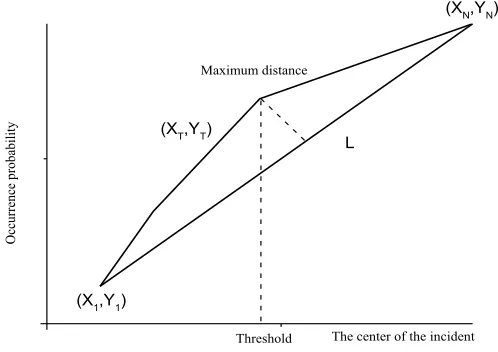
histogram may still fluctuate drastically. Even so, the cumulative histogram is an increasing function or a monotonically increasing function because the cumulative histogram accumulates all sampling points or the occurrence of a portion of sampling points for each sampling point. Cumulative histograms don’t fluctuate. From this point of view, finding the threshold in the cumulative histogram can reduce the inflection point to find a trend that indicates a rapid shift in the cumulative occurrence rate. Inflection points are mainly used for time series analysis and statistical process control. Because the cumulative histogram shows the rate of occurrence of a series of events, by analyzing a cumulative histogram to extract the inflection point where the ratio trend occurs, it can be used to divide the cumulative histogram or event into two parts: motion and no motion.
Fig. 2. Inflection point of cumulative histogram
The process of finding the inflection point of the cumulative histogram is as follows. Assume that there are N events in the cumulative histogram, the center of event i is Xi, and the occurrence ratio of event 1 is Yi, where 1≤i≤N. The straight line L connecting (Xi, Yi) and (XN, YN) is the accumulation of the equilibrium histogram. Therefore, the distance from each point (Xi, Yi) to the straight line L reflects the cumulative difference in event points with respect to the cumulative histogram accumulated value, where 2≤i≤N−1. Therefore, building a watershed from the maximum distance from the event point to the line divides the cumulative histogram into two parts: the distance from the event point to the line L gradually increases, and the distance from the event point to the line L gradually decreases. In other words, the trend of the distance to the straight line L changes at the point where the distance is the largest. Therefore, the maximum distance point (XT, YT) to the straight line L, that
Occurrence p
rob
abilit
y
The center of the incident
L (XT,YT)
(XN,YN)
(X1,Y1)
is, the hanging point can be used as the threshold, and XT is the selected threshold, as shown in Figure 3.
The line L can be derived from the following equation:
. (8)
Assume that the resulting linear equation is:
. (9)
Then the distance from the point (Xi, Yj) to the line L is:
. (10)
Compare the distance of all points (Xi, Yj) to the straight line L, where 2≤i≤N-1, set to:
. (11)
Therefore, the selected threshold is XT. The computational complexity of selecting a threshold from the cumulative histogram is 2) multiplication operations, 2*(N-2) addition operations, (N-2*(N-2) absolute operations, and (N-3) comparison operation, where N is the number of event points in the cumulative histogram.
Since the calculation time of the threshold selection is linear with the number of event points, the proposed threshold selection method is very effective. If the difference pixel value or the ratio pixel value is less than or equal to XT, it is regarded as a pixel without motion, and if the difference pixel value or the ratio pixel value is larger than XT, it is considered as a motion pixel. The steps for selecting a threshold are as follows:
A cumulative histogram of the target image is calculated, and the center and the appearance ratio of the event point are represented by coordinate points in the cumulative histogram, and all the points are arranged in ascending order.
The linear equation connecting the first point and the last point is calculated, and the distance from all points to the straight line except for the first point and the last point is calculated.
The event point with the largest distance to this straight line is selected as a threshold, and a pixel smaller than or equal to the threshold is regarded as a pixel without motion, and a pixel larger than the threshold is regarded as a motion pixel.
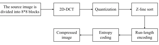
Low complexity JPEG encoding algorithm
The JPEG encoding process is shown in figure 4. Firstly, the source image is divided into a number of 8*8 blocks, then each block is subjected to DCT transformation, and a unified quantization table is used to quantize the transformed
)
(
)
(
)
(
)
(
1 1 1
1
N N
X
X
Y
Y
X
X
Y
Y
-=
-0
*
*
a
X
+
b
Y
-
c
=
2 2
j
i
b
*
Y
c
|
X
*
a
|
b
a
+
+
+
)
),
,
((
max
arg
N-12
i
D
X
Y
L
coefficients. Then, the quantized results are arranged in a zigzag sequence in ascending order of frequency, and the length of the sequence is reduced by run length coding. Finally, entropy coding is performed for further compression.
Fig. 3. JPEG encoding process
The forward transformation formula is as follows
. (12)
Among them, .
u, v is a discrete frequency variable, where 0≤u, v≤k−1, k is the size of the DCT block. f(x, y) is the gray value of the pixel point (x, y) in the N*N image, where 0 ≤ x, y ≤ k - 1, which is the coefficient of the point (u, v). F (u, v) is the coefficient of the point (u, v).
For the reference frame, in order to maintain its image quality, all 64 DCT coefficients are calculated, and the fast approximation calculation method is used to reduce the computational complexity. The calculation formula is as follows:
. (13)
Where, [x] is the largest integer less than or equal to X. Although the approximation calculation will introduce errors, due to the large quantization step after DCT, this error will not have any effect.
For the current frame captured by the video node, different processing methods are adopted according to different DCT blocks to ensure the image quality of the changed area. For blocks marked static or no noise, no DCT operation is performed and all coefficients are set to zero; for blocks that are marked as moving, DCT is used to
The source image is
divided into 8*8 blocks 2D-DCT Quantization Z-line sort
Run-length encoding Entropy coding Compressed image
åå
= -=+
=
1 -k 0 x 1 0]
2
)
1
2
(
cos
)
,
(
[
*
)
(
)
(
2
1
v
u
k yk
u
x
y
x
f
v
C
u
C
k
F
p
)
,
(
otherwise
v
C
C
v
u
for
v
C
C
(
u
),
(
)
=
1
/
2
,
=
0
;
(
u
),
(
)
=
1
16
)
1
2
*
2
(
2
cos
16
)
1
2
*
2
(
2
cos
*
)
,
(
[
*
4
1
)
,
(
7 4 7 4p
p
y
v
approximately calculate combined clipping optimization, 4*4 low frequency DCT coefficients are calculated, and the other coefficients are zeroed.
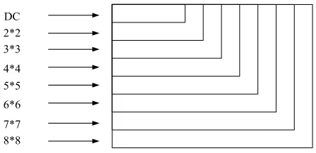
The most valuable information in the image is usually stored in the low frequency part of the DCT. After quantization, many DCT high frequency coefficients become zero. Therefore, only the 4*4DCT low-frequency coefficients containing the main energy of the image need to be calculated, and the other 48 coefficients are set to zero, which can also reduce the computational complexity of the quantization stage.
Fig. 4. Square DCT coefficient block
As shown in Figure 5, if only the partial coefficients of k*k (k=1, ..., 8) in 2-D DCT are calculated, the computational complexity will be reduced and the image reconstruction quality will also be reduced. The image content and the selected k jointly determine the image quality. The number of multiplications (M) and the number of additions (A) required for the N*N DCT are calculated by the following formula, where N is a power of two.
. (14)
. (15)
4
Simulation Experiments and Analysis
It is assumed that wireless multimedia sensor network is applied to regional monitoring and adopts layered structure, base station, cluster head node and common video sensor node. The video sensor nodes are evenly deployed and completely cover the monitoring area. All nodes are immovable and are battery powered. The video node is responsible for capturing and encoding the image of the surveillance area and transmitting the encoded image to the cluster head node.
Simulation experiment results
The test image sequence of the “PETS' 2000, 2000 IEEE International Workshop Performance Evaluation of Tracking and Surveillance” is simulated on MATLAB. The image scene is an outdoor parking lot. A high-positioned camera captured 1,452 frames of images in 58.08 seconds at a speed of 25 Hz. During this period, people and
DC 2*2 3*3 4*4 5*5 6*6 7*7 8*8
N
N
M
=
(
2/
2
)
log
22
2
log
)
2
/
5
(
2 2-
+
=
N
N
N
vehicles entered the surveillance area. The original image format is a 768*578 pixel color image.
Images of numbers 0000, 0120, 0130, 0140, 0150, 0160, 0180 are selected, and they are converted into SIF format, that is, a grayscale image of 320*240 pixels, and then an image coding algorithm is used for the simulation experiment.
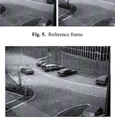
Fig. 5. Reference frame
Fig. 6. Current frame
Figure 6 (left) is 0000 frames selected as the reference frame and Figure 6 (right) reference frame uses DCT to approximate the JPEG algorithm compressed image. The image PNSR compressed by the JPEG standard algorithm is 36.1141, the PSNR of the DCT approximate calculation JPEG algorithm is 32.8226, and the approximate calculation causes a loss of 3.2915 dB. Figure 7 is the current frame numbered 0180 where a car is passing through the parking lot and a person is heading towards the parking lot.
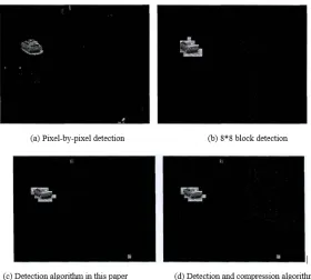
algorithm are shown in Figure 8(c). There is still a small amount of residual noise, but both the moving vehicle and the pedestrian are tested and the computational complexity is low. Figure 8(d) shows the detection result image after compression with the optimized JPEG algorithm.
Fig. 7. Comparison of change detection methods
Fig. 8. Results of change detection and compression
4.1 Calculation complexity analysis
Table 1. The operation times of additions and multiplications of 2D-DCT
2D-DCT Fast DCT DCT cropping 4*4
coefficients This article's algorithm Calculation of variation detection DCT approximation
Multiplication 96 96 48 48
Addition 466 312 112+15=127 112+65=117
The wireless sensor node platform Imote2 of American Krsbo Company is the advanced node platform at present, it has 256kb SRAM, it is the wireless transceiver device of 250kb/ s of transmission speed. If the size of a frame of image is 48 kb, and a 320*240 pixel monitor image is acquired at 25 Hz, 1200 kb of data will be generated in one second. when a 320*240 pixel surveillance image is acquired at 25 Hz, 1200 kb of data will be generated in one second. These image data exceed the storage capacity of the SRAM and the transmission capability of the radio. The node is unable to complete the data transfer task and consumes a lot of energy. After the change detection is performed, only the moving target is retained. As shown in Table 2, the detection result indicates that the image size of each frame is approximately 5 kb, much smaller than the original image. The image data generated in one second is only about 125kb. Imote2 can complete the data transmission task and can effectively save computing and communication energy consumption.
Table 2. Comparison of the size of the image after the change test with the original image
Image
number Full frame size Test results Ratio of test results to full frame size PSNR
0120 51.9k 6.15k 11.85% 25.35
0130 47.4k 6.16k 13.00% 26.44
0140 48.6k 5.50k 11.32% 28.47
0150 48.5k 5.13k 10.58% 29.40
0160 48.6k 4.71k 9.69% 29.01
0180 48.2k 4.85k 10.06% 27.40
Table 3. Comparison of change detection operations
Change detection
algorithm Pixel by pixel Block by Block Proposed algorithm
Addition(320*240) 320*240*2=153600 1200*(64+1)=78000 1200*(14+1)=18000
5
Conclusion
A low-complexity image coding algorithm based on change detection and optimized JPEG for WMSN is proposed. The change detection algorithm uses a single reference frame and detection threshold, which can effectively filter out most of the noise in the image, detect the moving target, and have a small amount of computation. Optimized DCT operations and quantized tables significantly reduce computational complexity at the expense of minimal image quality loss. Simulation experimental results show that the detection algorithm has high detection accuracy and effectively reduces the amount of data transmission. The optimized image coding algorithm effectively reduces the computational complexity and guarantees the image quality.
6
References
[1]ZainEldin, H., Elhosseini, M. A., & Ali, H. A. (2015). Image compression algorithms in wireless multimedia sensor networks: A survey. Ain Shams Engineering Journal, 6(2): 481-490. https://doi.org/10.1016/j.asej.2014.11.001
[2]AlSkaif, T., Bellalta, B., Zapata, M. G., & Ordinas, J. M. B. (2017). Energy efficiency of MAC protocols in low data rate wireless multimedia sensor networks: A comparative study. Ad Hoc Networks, 56: 141-157. https://doi.org/10.1016/j.adhoc.2016.12.005
[3]Costa, D. G., Guedes, L. A., Vasques, F., & Portugal, P. (2015). Research trends in wireless visual sensor networks when exploiting prioritization. Sensors, 15(1): 1760-1784.
https://doi.org/10.3390/s150101760
[4]Khan, M. A., Ahmad, J., Javaid, Q., & Saqib, N. A. (2017). An efficient and secure partial image encryption for wireless multimedia sensor networks using discrete wavelet transform, chaotic maps and substitution box. Journal of Modern Optics, 64(5): 531-540.
https://doi.org/10.1080/09500340.2016.1246680
[5]Usman, M., Yang, N., Jan, M. A., He, X., Xu, M., & Lam, K. M. (2018). A joint framework for QoS and QoE for video transmission over wireless multimedia sensor networks. IEEE Transactions on Mobile Computing, 17(4): 746-759.
https://doi.org/10.1109/TMC.2017.2739744
[6]Rault, T., Bouabdallah, A., & Challal, Y. (2014). Energy efficiency in wireless sensor networks: A top-down survey. Computer Networks, 67: 104-122. https://doi.org/10.1016/j .comnet.2014.03.027
[7]Ghadi, M., Laouamer, L., & Moulahi, T. (2016). Securing data exchange in wireless multimedia sensor networks: perspectives and challenges. Multimedia Tools and Applications, 75(6): 3425-3451. https://doi.org/10.1007/s11042-014-2443-y
[8]Jiang, D., Xu, Z., Li, W., & Chen, Z. (2015). Network coding-based energy-efficient multicast routing algorithm for multi-hop wireless networks. Journal of Systems and Software, 104: 152-165.
[9]Gonçalves, D. D. O., & Costa, D. G. (2015). A survey of image security in wireless sensor networks. Journal of Imaging, 1(1): 4-30. https://doi.org/10.3390/jimaging1010004
[10]Kidwai, N. R., Khan, E., & Reisslein, M. (2016). ZM-SPECK: A fast and memoryless image coder for multimedia sensor networks. IEEE Sensors Journal, 16(8): 2575-2587.
[11]Rein, S., & Reisslein, M. (2016). Scalable line-based wavelet image coding in wireless sensor networks. Journal of Visual Communication and Image Representation, 40: 418-431. https://doi.org/10.1016/j.jvcir.2016.07.006
[12]Han, G., Jiang, J., Guizani, M., & Rodrigues, J. J. C. (2016). Green routing protocols for wireless multimedia sensor networks. IEEE Wireless Communications, 23(6): 140-146.
https://doi.org/10.1109/MWC.2016.1400052WC
7
Authors
Jie He is a Researcher of Department Of Electronic Information Engineering Of ChongQing Technology And Business Institute, ChongQing, 401520, China. His research interests include JPEG Image Coding Algorithm.