Multiple-View Active Learning for
Environmental Sound Classification
https://doi.org/10.3991/ijoe.v12i12.6458
Yan Zhang, Danjv Lv and Yili Zhao
Southwest Forestry University, Kunming, China
Abstract—Multi-view learning with multiple distinct feature
sets is a rapid growing direction in machine learning with boosting the performance of supervised learning classification under the case of few labeled 1data. The paper
proposes Multi-view Simple Disagreement Sampling (MV-SDS) and Multi-view Entropy Priority Sampling (MV-EPS) methods as the selecting samples strategies in active learning with multiple-view. For the given environmental sound data, the CELP features in 10 dimensions and the MFCC features in 13 dimensions are two views respectively. The experiments with a single view single classifier, SVML, MV-SDS and MV-EPS on the environmental sound extracted two of views, CELP & MFCC are carried out to illustrate the results of the proposed methods and their performances are compared under different percent training examples. The experimental results show that multi-view active learning can effectively improve the performance of classification for environmental sound data, and MV-EPS method outperforms the MV-SDS.
Index Terms—Active learning; Multiple-view learning;
MV-SDS; MV-EPS
I. INTRODUCTION
Audio classification is an important access to extract audio structure and content, as well as a basis for audio retrieval and analysis. The environmental sound classification is attracting the attention of researchers increasingly [1]. Classification model selection has been the focus in the speech recognition and classification. The existing techniques for audio classification, such as minimum distance classifier, neural network, support vector machines, decision tree, and hidden Markov Model [2], have proven their efficiency for handling audio data. Li Yong et al. [3] combined the stream learning with SVM, which obtained the performance of classification efficiently and accurately for ecological environmental sound data. But it is difficult to find the optimal classifier with good generalization and to improve the performance of supervised classifier.
In the actual application, the performances of supervised algorithms strongly depend on the representativeness of the data used to train the classifier. This constraint makes the generation of an appropriate training set, a difficult and expensive task requiring extensive manual analysis for the environmental audio data. The classification of environmental audio requires a number of training examples that are too expensive or
1This work was supported by the national natural science foundation of
China under the Grant No. 61462078
tedious to acquire. With the number of the labeled examples decreases in the supervised classification, the performance will get worse. It is difficult for traditional supervised classification (passive learning) to construct the classifier model to meet the accuracy requirement. Those emerging approaches are focus on to obtain better classification accuracy under the condition of a few labeled samples and a number of unlabeled examples [4-6].
So more researches focusing on higher accurate rate can be obtained based on the few labeled and lots of unlabeled examples [4-5]. In machine learning fields, ensemble [7] can effectively deal with this issue. How to use a few labeled data to improve the learning performance becomes the key problem, which the pattern recognition and machine learning researchers are focusing on.
For the environmental sound data with few labeled samples, it is a good way to combine various algorithms and exploit complementary between different classifiers to boost the classification accuracy of environmental sound. The literature [7] exploited ensemble technologies including Bagging, AdaBoost, Random Forests and MCS (multiple Classifier System), combination of different single classifiers. That can obtain better performance than any other single classifiers. Semi-supervised learning and active learning, as methodologies of machine learning, make the best use of the unlabeled samples to assist the few labeled examples in establishing classifier model to improve the performance of classification even under the fewer number of the training examples. Zhang Yan et.al proposed EPS (Entropy Priority Sampling) and SDS(Simple Disagreement Sampling) methods as the selecting sampling strategies in active learning[8]. For the given environmental sound data, the CELP features in 11 dimensions are extracted. The experiments with the single classifier, EPS and SDS on the environmental sound are carried out in order to illustrate the results of the proposed methods and compare their performance under different percent training sample. The experimental results show that active learning can effectively improve the performance of environmental sound data classification, even under the fewer number of the training examples. The EPS method outperforms the SDS. The literature [9] combined support vector machines (SVM) and EPS, and presented the SVM_EPS methods as the selecting strategy in active learning for environmental audio data classification.
classifier trained on a small set of well-chosen examples can perform as well as a classifier trained on a larger number of randomly chosen examples. Therefore, active learning is proposed to effectively deal with this issue. In active learning, the learner actively selects the unlabeled samples with most information, and then the experts label them. The new labeled examples are joined the training sets to enlarge the training sets, so as to acquire better performance, and decrease the cost to construct the classification model [10].
The remainder of the paper is organized as follows. Section 2 presents the general framework of active learning and briefly reviews some related work with multiple views learning. Section 3 presents two approaches to multiple views with active learning. Section 4 gives two views features of environmental audio dataset considered in the experiments. Section 5 compares the different approaches numerically in experimental results. Finally, section 6 concludes and issues some future work.
II. ACTIVELEARNINGANDMULTIPLEVIEWS
A. Active Learning
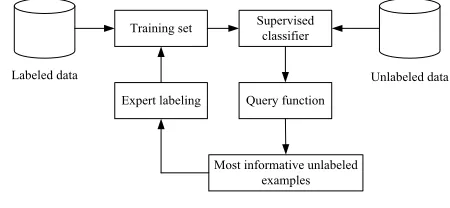
The professor Angluin of Yale University first put forward the concept of active learning [11]. In active learning, the learning process repeatedly queries unlabeled samples to select the most informative examples and updates the training set on the basis of a supervisor who attributes the labels to the selected samples. The query function samples from the unlabeled pool, which have maximum ambiguity to belong to each class. The following chart of the general active learning is showed in Fig.1.
Training set
Labeled data
Supervised classifier
Query function
Most informative unlabeled examples Expert labeling
Unlabeled data
Fig. 1 Description of general active learning
Active learning algorithms are iterative sampling schemes, where a classification model is adapted regularly by feeding it with new labeled examples corresponding to the ones that are most beneficial for the improvement of the classification model performance. The examples are usually found in the areas of the uncertainty of the model and their inclusion in the training set forces the model to solve the regions of low confidence.
An active learning process requires interaction between the user and the model: the former provides the labeled information and the knowledge about the desired classes, while the latter provides both its own interpretation of the distribution of the classes and the most relevant examples needed to solve the discrepancies encountered. This point is crucial for the success of an active learning algorithm [12]: the machine needs a strategy to rank the examples in the unlabeled examples pool. These strategies, or heuristics, differentiating the algorithms can be divided into three main families:
1) Committee-based heuristics [13],
2) Large margin-based heuristics [14], 3) Posterior probability-based heuristics [15].
The committee based on active learning methods quantifies the uncertainty of a sample by considering a committee of learners. Each member of the committee exploits different hypotheses about the classification problem and consequently labels the samples in the pool of unlabeled candidates. The algorithm then selects the samples showing maximal disagreement among the different classification models in the committee which speeds up the learning process. It will achieve the better performance and reduce the cost of the manual labeling with a few labeled training set.
B. Multiple Views Learning
Blum and Mitchell[16] provided the first formalization of learning in the multi-view framework, and proved that two independent, compatible views can be used to PAC-learn[17], a concept based on few labeled and many unlabeled examples. At the meantime, they also introduced Co-Training, the first general-purpose, multi-view algorithm.
In the traditional single-view machine learning, a learner has to access to all set of domain features. By contrast, in the multi-view setting the domains features can be partitioned in subsets. Each subset, i.e. each view is sufficient for learning the target concept to build the classifier model. In the multi-view learning, every example is described by a different set of features in each view. For example, V1,V2,..,Vk are k views in a domain
features, a labeled sample can be presented as the tuple <x1,x2,…,xk,y>, where y denotes label, and x1,x2,…,xk are its feature descriptions in the k views. The unlabeled sample is denoted by <x1,x2,…,xk,?>, where ‘?’ denotes the unknown label.
In general, the research of active learning focuses on main two aspects including multi-view or single-view and multi-classifier or single-classifier. The algorithms fall under four main categories: SVSL(Single View Single Learner), SVML(Single View Multiple Learners)
MVSL(Multiple View Single Learner), and MVML(Multiple View Multiple Learners) [18].
III. MULTI-VIEWACTIVELEARNING
A. Multiple View Single Learner (MVSL)
In MVSL, two different classifiers h1, h2are obtained from two different views Vi and Vj with same learning algorithm H. Then, the unlabeled examples are predicted with classifier hi and hj. The condition of the labeling the unlabeled example is equation (1).
"
!
!
(1)The contention points (CPs) can be selected by disagreement between the two classifiers of the prediction results. The approach is named as MV-SDS (Multi-view Simple Disagreement Sampling). Fig.2 shows the description of the MV-SDS, in which two different views are involved.
Fig. 2 Description of MV-SDS algorithm
B. Multiple View Multiple Learner( MVML)
MVML active learning selects the most informative examples to label. Two aspects of disagreement are considered. One is the disagreement among the different views, and the other is the disagreement of the prediction results with multi-classifiers in each view. Combing the two disagreements, the condition of sampling the examples from the unlabeled pool can be reached.
DisAll=Diff1+Diff2 (2)
Diff1 comes from the difference among the views. For each example from the unlabeled pool, the predicted results are disagreement in different views.
}
),
(
)
(
and
|
{
1
x
x
U
h
x
h
x
i
j
Diff
=
"
i!
j!
(3)Where histands for the classifier model trained by the training dataset from the Vi. So does hj.
Diff2 describes the difference in each view. The
measure of it is the average of the disagreement in each view.
!
==
(4)
DisVi can be measured by the entropy of the classifications voted by each member classifier in the view. The detail of obtaining DisViis as follows.
Given k different classifiers, committee-based sample selection techniques are applied to select examples from unlabeled pool for training. Disagreement among the k
committee members can be measured by the entropy of the classifications voted by each member. For one example as x, the entropy value in one view is computed by the equation (5) an (6).
!
= " =
(5)
= (6)
Where Vote(i) is the number of votes of class i, c is the total number of classes. Examples corresponding to higher entropy have priority of selection over others. When the
Ent(x) is obtained in i-th view, that is the DisVi.
In the process sampling of MVML, the contention points are firstly selected from the disagreement among the views. Then, the entropy of classifications voted
EntVi(x) is computed by each member in i-th view, corresponding to above the DisVi. The final entropy of the sample point x under m views is acquired by equation (7).
!
= =
(7)
Fig. 3 Description of MV-EPS algorithm
Algorithm: MV-SDS
Input: L--Labeled examples, U--Unlabeled examples H--learning algorithm, N--number of iteration V1,V2--two different views
Output: Hout final classifier
Loop for N iterations
// Use L to learn the classifiers in the views V1,V2 h1=H(L from V1);
h2=H(L from V2);
! " CPs ;
For each xi!Udo
)} ( ) ( and |
{ CPs
CPs# ! xi xi"U h1 xi !h2 xi ;
U !U-{CPs}; // remove CPs from the U
NewL!Label (CPs); // label the contention points
L
!
L
!
NewL
;End Loop
Hout= Ensemble (h1, h2)
Algorithm: MV- EPS
Input: L-- Labeled examples, U--Unlabeled examples Hk(k"3) --: learning algorithm, k--number of Hk
N--number of iteration,V1,V2-- two different views,
n--number of sampling in each iteration Output: Hout final classifier
Loop for N iterations
= ; (i=1...k,k"3)
= ; (j=1...k,k"3)
//ensemble the different classifiers in one view h1=ensemble(
h
k1);h2=ensemble(h
k2);! "
CPs ;
For each xi!Udo If h1(xi)!h2(xi) Then {
EntV1(xi)=entropy of xi for V1;
EntV2(xi)=entropy of xi for V2;
Ent(xi)=mean(EntV1(xi),EntV2(xi));
i
x
!
CPs CPs! ; }
Sort CPs in decreasing order of Ent(xi) ; S! CPs[1..n] ; //select the top n CPs U !U-S; // remove S from the U
NewL!Label (S); // label the contention points L!L! NewL;
End Loop
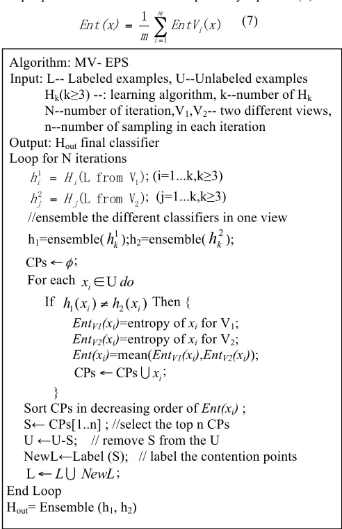
Finally, according to the descending order of the Ent(x)
value, the top n points are determined and labeled to move into the training set. This is a round iteration. N iterations can be implemented to meet some constrains .The approach is named as MV-EPS (Multi-view Entropy Priority Sampling). The description is illustrated in Fig 3.
C. Construction of Multiple Views Views
The key point of multiple-view learning is how to construct k views (k"2). According to the idea of literature [24], three methods are exploited to to solve this issue.
1) Random Features Split: The all features in a V view, are divided into k sub-space, such as V1,V2,..,Vk. For
instance, to generate two views, there are
!
"
= ,= !. The features of each view are randomly selected from V, and meets
! =
! .
2) Extracting Features Split: According to the different methods of extracting features, different views are formed. 3) Features Importance Split: During the building of classification mode based on training dataset, the contribution to classification of the feature variable can measured by the variable importance metric. Especially, for random forests method, the rank of the feature importance can be obtained by Mean Decrease Accuracy or Mean Decrease Gini. The multiple views can be generated by divided the ordered features. For two views, one view comes from the odd order of features, and the other is the even order of ones.
IV. EXPERIMENTDATAANDMETHOD The experimental data are acquired from network and field recording, with 8k sampling rate, 16 bits and mono-track. The environmental sound data includes five classes, such as the sound of different kinds of birds, frogs, wind, rain and thunder. The sound audio length amounts to almost 10 minutes. The silence and noise are removed in the pre-processing.
A. Feature Extraction of Environmental Audio
The feature extraction is executed based on the bit-stream through the G.723.1 data encoding on the Matlab platform. CELP and MFCC features are extracted respectively. There, Extracting Features Split method is adopted to construct the two views, CELP as V1 where
MFCC as the other V2. CELP is characterization by
coefficient of short tube cascade channel model, while MFCC is based on human auditory representation speech signal characteristics by means of frequency conversion.
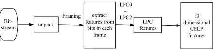
CELP features are mainly from LPC, that is, Linear Prediction Coefficient, which analyzes the sound mechanism from the original source. Through the short tube of channel cascade model research, the system transfer function is in line with the pile in the form of digital filter, so the signal of t time can be used several times before combination of the signal to estimate. By making the actual speech samples values and linear prediction to achieve minimum mean square error between the sampling value LMS. The linear prediction coefficients can be obtained.
Bit-stream unpack
extract features from
bits in each frame
LPC features
10 dimensional
CELP features Framing
LPC0 ~ LPC2
Fig. 4 Composed CELP audio features
LPC features are extracted at each bit-frame after the unpacked bit-stream. 10 order coefficients of LPC is obtained at each bit-frame, from 0 ~ 23bit (LPC0 ~ LPC2), which consists of the 10 dimensions of LPC features.
The other view is the features named MFCC (Mel-scale Frequency Cepstral Coefficients). The human ear is sensitive to the frequency of different levels. That is, it has the strong recognition ability for the low frequency of the voice signal while weak for the high frequency signal. The bit-streams of the data are transferred into the wave format. With the compression features of MFCC, the features extracting process is as below.
1) To transfer the signals of environmental audio data from time domain to frequency domain with FFT (Fast Fourier Transform);
2) Convolution of the logarithmic energy spectrum of signals in accordance with Mel scale distribution in triangular filter;
3) The vector composed of each filter output is transferred with DCT (Discrete Cosine Transform), taking the top 13 coefficients.
Fig.5 shows the detail process of the extracting MCFF features.
Fig. 5 Process of extracting MFCC features
B. Method of Experiments
The experiment is carried out on the platform of development Weka[25]. At first, the environmental audio feature data and training dataset are converted to the ARFF format files through program of Matlab. Then the ARFF format file can be obtained and classified with the module in development Weka. Finally, the results are obtained in ARFF file.
Encoded Enviromental
Audio Feature extraction
Convert to ARFF file
Recognition
Results Develop on Weka
Fig. 6 Flow chart of environmental audio classification
Pre-Processing Cutting Audio Hamming window FFT Filters
Tri-DCT
MF CC
Time-domain
V. ANALYSISOFEXPERIMENTALRESULTS
The frame of the environmental audio data is the basis unit for data statistics and classification in the experiments. In order to avoid large amount of data overflowing in training, the experimental data are selected from the total number of frames in the sampling according to one-third of the total data in each category. It is 10 times sampling randomly with 75% as the training sample, 25% as the testing sample. Finally, the result is the average of classification of the 10 times. Five classes of audio signal frame situation and classification of samples are shown in TABLE I.
TABLE I INFORMATION OF DATASETS IN THE EXPERIMENTS
class Total frames 75%--training 25%--test
bird 2277 1708 569
wind 9401 7051 2350
rain 9092 6819 2273
frog 4459 3344 1115
thunder 2451 1838 613
total 27680 20760 6920
In order to show the performances of different methods proposed in the paper, the rate of training examples are 10%,20%,40%,60% and 80% respectively. Three classification methods including traditional SVML, MVSL and MVML are compared in the experiments. The single learner adopts the decision tree J48. J48 (Decision tree) and RBF (Radial Basis Function) are applied in the SVML to select the disagreement points from the unlabeled pool. MVSL uses MV-SDS presented above in this paper, and the sampling classifiers are J48 and RBF, respectively. MV-EPS method is used in the MVML with each view exploring three different classification approaches such as J48, RBF and NB (Naïve Bayesian) to select the most informative examples. The examples of training data in each group are picked randomly according to the rate of total unlabeled samples. The experimental results are the average of the ten times run. The average results involved those methods are summarized in TABLE II, which present the classification accuracy of the methods i.e. SVSL, SVML, MV-SDS and MV-EPS.
TABLE II CLASSIFICATION AVERAGE ACCURACY RATES UNDER DIFFERENT PERCENT LABELED SAMPLES
Training samples rate
SVSL
SVML
MVSL MVML
View1 View2 MV-SDS MV-EPS
10% 87.540% 87.999% 90.728% 92.249% 94.413% 20% 90.416% 89.397% 91.569% 94.055% 95.337% 40% 91.594% 90.100% 92.143% 95.283% 96.101% 60% 91.683% 90.789% 92.699% 95.977% 96.272% 80% 92.159% 91.316% 92.688% 96.103% 96.468%
In the TABLE II, both the column view1 and view2 presents the accuracy rate of each view with single classifier J48. From the experimental results, the performances of the SVML, MV-SDS and MV-ESP outperform that of the SVSL (single view with one supervised classifier). For the active learning, MVSL is better than SVML, which shows the merit of the multiple views in classification with environmental audio data. And under the case of the multiple views, the MV-EPS is super to the MV-SDS. It is quite clear that among the data TABLE II, the performance of MV-EPS is best. In this approach, the strategy of select examples from unlabeled pool considers the disagreement with the two views, as well as that among the different classifiers in each view. The chosen contention points, through two aspects of disagreement, enlarge the number of training examples and enrich the information of constructing the classification model. But the disagreement between the two views is involved in the sampling strategy.
For example, under the case of the 10 percent labeled examples as training data, MV-SDS obtained the accuracy of 92.249%, and 94.41% for MV-EPS, while 92.159% of single view single classifier with 80 percent labeled examples. Active learning with multiple views explores fully the most informative unlabeled examples to reduce the amount of the training samples that satisfies the supervised classifiers and effectively improves the classification performance under different rates of the labeled data.
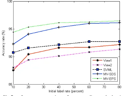
Fig.7 shows the performance of corresponding methods of experimental data. Generally, MV-SDS and MV-EPS outperform other approaches, obviously shown in the curve variation of MV-SDS, but under the less training samples (between 10% and 40%), the accuracy of MV-EPS is higher than that of MV-SDS. Therefore, multiple-view in classification works is better than the single multiple-view. Although the curve of SVML is higher than that of the single view single classifier, performance is not improved obviously with the increasing the amount of the training examples.
Fig.7 performance comparison of corresponding methods with environmental audio data
learner retrained at each iteration could contain many noises and the mislabeled examples will keep on affecting the learner in the subsequent iterations. The data editing approach [26] can solve the problem.
VI. CONCLUSION
How to leverage the abundant unlabeled data with a few labeled training examples to construct a strong classification system is a focus issue. The classification of environmental audio requires a number of training examples that are too expensive or tedious to acquire. Active learners alleviate the burden of labeling large amounts of data by detecting and asking the user to label only the most informative examples in unlabeled pool. In this paper, we focus on active leaning with multiple-view, referring several subsets of features. Based on the introduction of multiple views learning, two approaches of multiple-view with active learning, SDS and MV-EPS, are proposed in the paper. They differ in the selecting samples strategies from the unlabeled pool. The disagreement among the different views is only considered in MV-SDS. Instead, the disagreement in the different views, as well as that among the different classifiers in each view is involved in the MV-EPS.
The experiments are carried out on the environmental audio data, whose two different views are LPC features and MFCC features respective. The classification methods include SVML, MV-SDS and MV-EPS. The experimental results show that the multiple views with active learning obtains better performance than that of the single view. Between the two approaches of the multi-views, the MV-EPS is super to MV-SDS.
Increasing diversity is the key to selective sampling in active learning, and a more extensive study needs to be done to employ the diverse ensemble in active learning. Further research work about the effectively exploiting the information from the unlabeled data with the active learning and the semi-supervised learning under the multiple views to build the better learning model are underway.
REFERENCES
[1] Zhang Xiaomei, Yang Dingcai. Environmental audio classification based on support vector machine[J]. Electronic-Measurement-Technology.2008,31(9):121-123.
[2] Yi-wen Zheng. Typical Methods for Audio-Classification[J].Ji Suan Ji Yu Xian Dai Hua. 2007,(8):59-63.
[3] Li Yong, Li Ying, Yu Qing-Qing. Environmental Sound Classification Based on Manifold Learning and SVM [J]. Computer Engineering.2011,37(7):288-290.
[4] Zhi-Hua Zhou, Yu Wang. Machine Learning and Application [M]. Beijing: Tsinghua University Press. 2007.
[5] Seeger,M. Learning with labeled and unlabeled data, Technical Report[R]. University of Edinburgh, Edinburgh, UK, 2001. [6] X.Zhu. Semi-supervised learning literature survey[R]. Technical
Report 1530, Department of Computer Sciences, University of Wisconsin at Madison, WI, Apr.2008.
[7] ZHANG Yan, LV dan-jv, WANG hong-song. The application of multiple classifier system for environmental audio classification. ICMIT 2013: proceedings of the 2013 International Conference on Mechatronics and Information Technology, Guilin, October 19-20, 2013[C]. Applied Mechanics and Materials, 2013.
[8] Zhang Yan, Lv Dan-Jv,Wang Hong-song. Research of Environmental Audio classification Based on Active Learning [J].Computer technology and development, 2014,24(6):110-113. [9] Yan Zhang, Danjv Lv, Ying Lin. Environmental Audio
Classification Based on Active Leanring with SVM [C].
In:Proceedings of the 2015 International Conference on Computer Science and Intelligent Communication.2015:208-212. https://doi.org/10.2991/csic-15.2015.50
[10] Liu Kang, Qian Xu,Wang Ziqiang.Survey on Active Learning Algorithms [J].Computer Engineering and Applications.2012,48(34):1-4.
[11] Angluin D. Queries and concept learning[J]. Machine Learning. 1998,2(4):319-342. https://doi.org/10.1007/BF00116828
[12] Wu Weining, Liu Yang, Guo Maozu, Liu Xiaoyan. Advances in Active Learning Algorithms Based on Sampling Strategy [J]. Journal of Computer Research and Development. 2012,49(6):1162-1173
[13] Seuong,H., Opper,M., Sompolinski, H. Query by committee[C]. In: Proceedings of the 5th ACM workshop on computational learning theory, Pittsburgh, PA, 1992:287-294.
[14] C.Campbell, N.Cristianini, A.Smola. Query learning with large margin classifiers. In Proc.ICML, Stanford, CA,2000:111-118 [15] N .Roy, A. McCallum. Toward optimal active learning through
sampling estimation of error reduction. In Proc. ICML, Williamstown, MA, 2001:441-448.
[16] Blum,A.,& Mitchell,T. Combiming labeled and unlabeled data with co-training. In Proceedings of the 1998 Conference on Computational Learning Theory. 1998:92-100.
[17] D.D.Lewis, A.W.Gale, A sequential algorithm for training text classifiers, in: proceedings of the 17th Annual International ACM SIGIR Conference on Research and Development in Information Retrieval, 1994,3-12. https://doi.org/10.1007/978-1-4471-2099-5_1
[18] Sun S, Zhang Q. Multiple-view multiple-learner semi-supervised learning [J]. Neural Processing Letters, 2011b,34:229-240. https://doi.org/10.1007/s11063-011-9195-8
[19] A.Dempster, N. Laird,D.Rubin, Maximum likelihood from incomplete data via the EM algorithm, Journal of the Royal Statistical Society, Series B 39. 1977:1-38.
[20] I.Muslea, S.Minton,C.Knoblock. Selective sampling +semi-supervised learning=robust multi-view learning, in Proceedings of the International Joint Conference on Artifical Intelligence,2001:435-442
[21] I.Muslea,S.Minton,C.Knoblock. Selective sampling with redundant views. In Proceedings of Association for the Advancement of Artificial Intelligence,2000:621-626.
[22] Y.zhou, J.Goldman. Democratic co-learning, in Proceedings of the 16th IEEE International Conference on Tools with Artificial Intelligence,2004:594-602
[23] Qingjiu Zhang, Shilinag Sun. Multiple-view multiple-learner active learning. Pattern Recognition. 2010,43:3113-3119. https://doi.org/10.1016/j.patcog.2010.04.004
[24] Sun S, Jin F, Tu W. View construction for multi-view semi-supervised learning [C]. Lecture Notes Computer Science, 2011a, 6675:595-601. https://doi.org/10.1007/978-3-642-21105-8_69 [25] Ian H. Witten, Eibe Frank, Mark A.Hall. Data Mining: Practical
machine learning tools and techniques (3rd ed.)[M]. Morgan Kaufmann, 2011
[26] DENG Chao, Guo MaoZu. ADE-Tri-Training:Tri-training with Adaptive Data Editing. Chinese Journal of Computer. 2007,30(8):1213-1226.
AUTHORS
Yan Zhang is with School of Computer and
Information, Southwest Forestry University, Kunming, China (e-mail: zydyr@ 163.com).
Danjv Lv is with School of Computer and Information, Southwest Forestry University, Kunming, China (e-mail: [email protected]).
Yili Zhao is with School of Computer and Information, Southwest Forestry University, Kunming, China (e-mail: [email protected]).