Bayesian Estimation Based on Record Values from Exponentiated Weibull Distribution: An Markov Chain Monte Carlo Approach

Published online January 20, 2015 (http://www.sciencepublishinggroup.com/j/ajtas) doi: 10.11648/j.ajtas.20150401.15

ISSN: 2326-8999 (Print); ISSN: 2326-9006 (Online)

Bayesian estimation based on record values from

exponentiated Weibull distribution: An Markov chain Monte

Carlo approach

Rashad Mohamed El-Sagheer

Mathematics Department, Faculty of Science, Al-Azhar University, Cairo, Egypt

Email address:

[email protected], [email protected]

To cite this article:

Rashad Mohamed El-Sagheer. Bayesian Estimation Based on Record Values from Exponentiated Weibull Distribution: An Markov Chain Monte Carlo Approach. American Journal of Theoretical and Applied Statistics. Vol. 4, No. 1, 2015, pp. 26-32.

doi: 10.11648/j.ajtas.20150401.15

Abstract:

In this paper, we consider the Bayes estimators of the unknown parameters of the exponentiated Weibull distribution (EWD) under the assumptions of gamma priors on both shape parameters. Point estimation and confidence intervals based on maximum likelihood and bootstrap methods are proposed. The Bayes estimators cannot be obtained in explicit forms. So we propose Markov chain Monte Carlo (MCMC) techniques to generate samples from the posterior distributions and in turn computing the Bayes estimators. The approximate Bayes estimators obtained under the assumptions of non-informative priors are compared with the maximum likelihood estimators using Monte Carlo simulations. A numerical example is also presented for illustrative purposes.

Keywords:

Exponentiated Weibull Distribution (EWD), Record Values, Bootstrap Methods, Bayes Estimation, Gibbs and Metropolis Sampler

1. Introduction

Record data and the associated statistics are of interest and importance in many areas of real life applications involving datd relating to meteorlogy, sport, economics, athletic events, oil, mining surveys and lifetesting. Many authors have studied records and associated statistics. Among them are Arnold et al. [1,2], Resnick [3], Raqab and Ahsanulla [4], Nagaraja [5], Ahsanulla [6,7], Raqab [8], Abd Ellah [9,10], Sultan and Balakrishnan [11], Preda and Panaitescu [12] and Mahmoud et al. [13]. Let X X1, 2,... be an infinite sequence

of independent identically (iid) continuous random variables (r.v.'s). An observation Xj will be called an lower record

value if Xj < Xi for every i< j . We will assume that Xj

occurs at time j , then the record time sequence is defined as,

0 1

T = and T_n =min{j:Xj <XTn−1}. The lower record value

sequence R0, R1, ..., Rn is defined as Rn = XTn ,n=0,1, 2,... . For more detail and references see Nagaraja [5], Ahsanullah [7] and Arnold et al. [2].

Mudholkar and Srivastava [14] introduced a two parameter Exponentiated Weibull distribution (EWD), an extension of

the well-known Weibull distribution. The beauty and importance of this distribution lies in its ability to model monotone as well as non-monotone failure rates which are quite common in reliability and biological studies. The form of the probability density function (pdf) and cumulative distribution function (cdf), with two shape parameters, α and

β

of the Exponentiated Weibull distribution denoted by

( , )

EWDα β are given, respectively, by

= − 1 − − , ›0, , ›0, (1)

= 1 − − , ›0, , ›0, (2)

of the performance of the different estimation methods in Section 6. Finally a conclusion is presented with some comments in Section 7.

2. Maximum Likelihood Estimation

In this section, we estimate α and

β

, by considering the maximum likelihood and we compute the observed Fisher information based on the likelihood equations. These will enable us to develop pivotal quantities based on the limiting normal distribution, the resulting pivotal quantities can be used to develop interval estimates. Suppose that ₍₁₎,

L x=x

( 2 ), L x ...,

( ) L n

x be the lower record values of size n from exponentiated Weibull distribution EWD( , )α β . The likelihood function for observed record x given by see Arnold et al. [2]

ℓ , | = ∏ !

" !

#$ , (3)

where f(.) and F(.) are given respectively, by (1) and (2), the likelihood function can be obtained by substituting from (1) and (1) in (3) and written as

ℓ , | =

% log )1 − − *+ ∏ !,-./ 0) !, *

/ 0) _!, *

#$ ,(4)

The logarithm of the likelihood function (4) is given by

1 , | = 2 log + 2 log + log )1 − − * +

− 1 4 log_#$ # − 5_#$ # −

5 log )1 −_#$ − # * . (5)

Differentiating (5) with respect to α and

β

and equating the results to zero, we obtain the likelihood equations for the parameters α and

β

as

7 , |

7 = − 4 log#$ # − 5_#$ # log # −

8 , − 9 #, = 0, (6)

where

8 , = − log

1 − −

and 9 #, = = !

, _{/ 0)}

!, * >?@ !

/ 0) _!, * , #$

(7)

7 , |

7 = − log )1 − − * = 0. (8)

The maximum likelihood estimate (MLE) of

β

say

β

ˆ , can be obtained as

A =

>?@B / 0) _C, *D, (9)

and the MLE of the α say ˆα can be obtained by solving the non-linear likelihood equation

= − 4 log_#$ # − 5 #

#$ log # + E C,

>?@B / 0) _C, *D− 9 #, , (10)

where

( )

( , ) L n

x

α

Φ and

( )

( , ) L i

x

α

Ψ are given in (7). Therefore, ˆ

α can be obtained as the solution of the non-linear equation in the form

ℎ = , (11) where

ℎ = 2

G H H H

I5 #

#$ log # − 4 log#$ # −

E C,

>?@B / 0) _C, *D+ 9 #, _JK

K K L

. (12)

Since ˆα is a fixed point solution of non-linear equation (10), therefore, it can be obtained by using a simple iterative scheme as follows

ℎ M = MN , (13)

where αj is the jth iterate of ˆα . The iteration procedure

should be stopped when |αˆj+1−αˆj | is sufficiently small.

Once we obtain ˆα from (10) , and the MLE of

β

say

β

ˆ becomes

A =

>?@B / 0) _C,O *D. (14)

2.1. Observed Fisher Information

The asymptotic variances - covariance of the MLEs for parameters α and

β

are given by elements of the inverse of the Fisher information matrix

IQR= S %− 7

T

7 7 + , U, V = 1,2. (15)

Unfortunately, the exact mathematical expressions for the above expectations are very difficult to obtain. Therefore, we give the approximate (observed) asymptotic variance-covariance matrix for the MLEs, which is obtained by dropping the expectation operator E

X_{]^_ A, \,}YZ[ \ ]^_ \, A_{YZ[ A} ` = a

7T _{, |}

7 T 7

T _{, |}

7 7 7T _{, |}

7 7

7T _{, |}

7 T

b , (16)

7T , |

7 T = − T− 5_#$ # log # c− d , −

e #, , (17)

where

d , = C, / 0) C, * >?@ CT% C, / 0) C, *+

% / 0) _C, _*+T , (18)

e #, = !

, _{/ 0)}

! , _{* >?@}

!T% !, / 0) !, *+

% / 0) _!, *+T , (19)

7T , | 7 7 =

7T , |

7 7 = 8 , , (20)

where 8 , is given in (7)

7T , |

7 T = T. (21)

The asymptotic normality of the MLE can be used to compute the approximate confidence intervals for parameters

,

α and

β

. Therefore, (1−δ)100% confidence intervals for parameters α, and

β

become, respectively, as

\ ± gh/cjYZ[ \ Z2k A ± gh/clYZ[ A , (22)

where g_h/c is the percentile of the standard normal distribution with right-tail probability m/2.

3. Bootstrap Confidence Intervals

In this section, confidence intervals based on the parametric bootstrap methods are proposed (i) percentile bootstrap method (Boot-p) based on the idea of Efron [15]. (ii) bootstrap-t method (Boot-t) based on the idea of Hall [16]. The algorithms for estimating the confidence intervals using both methods are illustrated as follows

3.1. Percentile Bootstrap Method

Algorithm 1

From the original data

(1), L x=x

( 2 ), L x ...,

( ) L n

x compute

the ML estimates of the parameters α⌢ and

β

⌢ by (10) and (14).

Use α⌢ and

β

⌢ to generate a bootstrap sample

(1), L

x∗ ₌x∗

( 2 ), L x∗ ...,

( ) L n x∗ .

As in Step 1, based on x∗ compute the bootstrap sample

estimates of α and

β

, say

α

⌢∗ and β⌢∗.

Repeat Steps 2-3 N times representing N bootstrap MLE's of ( , )α β based on N different bootstrap samples.

Arrange all

α

⌢∗′s and β⌢∗′s, in an ascending order to obtain the bootstrap sample ( [1]_,

l

φ [2]_,

l

φ _..., [N]_),

l

φ

1, 2

l= (where φ α φ₁ ≡⌢∗, ₂ ≡β⌢∗).

Let G z( )=P(φl ≤z) be the cumulative distribution function of φ₁. Define φ_lboot=G−1( )z for given z. The approximate bootstrap 100(1−δ)% confidence interval of φ_l is given by

%nopqqr)h_c* , nopqqr) _ch*+. (23)

3.2. Bootstrap-t Method

Algorithm 2

From the original data

(1), L x=x

( 2 ), L x ...,

( ) L n

x compute

the ML estimates of the parameters α⌢ and

β

⌢ by equations (10) and (14).

Using α⌢ and ⌢

β

generate a bootstrap sample

(1) (2) ( )

{x_L∗ ,x_L∗ ,...,x_{L n}∗ }. Based on these data, compute the bootstrap estimate of α and

β

using (10) and (14), say

⌢

α

∗ and β⌢∗ and following statistics

s∗₌√ O∗ O

jvwx O∗ Z2k sc∗=√ y

∗ y

lvwx y∗ ,

where YZ[ \∗ and YZ[ A∗ are obtained using the Fisher information matrix.

Repeat Step 2, N boot times.

For the T₁∗ _and T₂∗ values obtained in Step 2, determine the upper and lower bounds of the 100(1−δ)% confidence interval of α and

β

as follows: let

( ) ( _i ), 1, 2

H x =P T∗≤x i= be the cumulative distribution function of T₁∗ and T₂∗. For a given x, define

\pqqr r _{= \ + 2} /c jYZ[ \ z

Z2k Apqqr r _{= A + 2} /c lYZ[ A z .

Here also, YZ[ \ and YZ[ A can be computed as same as computing theVar(α⌢∗) and Var(β⌢∗) . The approximate 100(1−δ)% confidence interval of α and

β

are given by

% \pqqr r)h_c* , \pqqr r) _ch*+ Z2k % Apqqr r)h_c* , Apqqr r) _ch*+.(24)

4. Bayes Estimation using MCMC

posterior density function and in turn compute the Bayes point estimates and also construct the corresponding credible intervals based on the generated posterior samples. By considering model (1), assume the following gamma prior densities for α and

β

as

{ |Z, | = }~

•

€ w | U ≥ 0

0 U < 0ƒ, (25)

and

{c |„, k = }

…†

€ ‡ ‡ k U ≥ 0

0 U < 0ƒ. (26)

The joint prior density of α and

β

can be written as

{ , = { |Z, | {c |„, k

=_{€ w € ‡}~•…† w ‡ _{−| − k . (27)}

Based on the likelihood function of the observed sample is given by (4) and the joint prior in (27), the joint posterior density of α and

β

given the data, denoted by {∗ , | , can be written as

{∗ _{, | =} ℓ , | ׉ ,

Š Š ℓ , | ‰ , ‹ …_•Œ _•Œ . (28)

Therefore, the Bayes estimate of any function of α and

β

say g( , )α β , under squared error loss function is

Ž• , = S , |…wrw Ž , =Š Š • , ℓ , | ‰ , ‹ …

Œ • Œ •

Š Š ℓ , | ‰ , ‹ …_•Œ _•Œ . (29)

Generally, the ratio of two integrals given by (29) cannot be obtained in a closed form. In this case, we use the MCMC method to generate samples from the posterior distributions and then compute the Bayes estimator of g( , )α β under the squared errors loss (SEL) function. Therefore, we propose the approaches of MCMC technique to approximate (29). See, for example, Robert and Casella [21] and, Rezaei et al. [22].

4.1 MCMC Technique

In this subsection we consider the MCMC method to generate samples from the posterior distributions and then compute the Bayes estimates of the parameters α and

β

under the squared errors loss (SEL) function. A wide variety of MCMC schemes are available. An important sub-class of MCMC methods is Gibbs sampling and more general Metropolis-within-Gibbs samplers. The advantage of using the MCMC method over the MLE method is that we can always obtain a reasonable interval estimate of the parameters by constructing the probability intervals based on the empirical posterior distribution. This is often unavailable in maximum likelihood estimation. Indeed, the MCMC samples may be used to completely summarize the posterior uncertainty about the parameters through a kernel estimate of the posterior distribution. This is also true of any function of the parameters.

The expression for the joint posterior can be obtained up to proportionality by multiplying the likelihood with the joint prior and this can be written as

{∗ _{, ∝} Nw N‡ _{%− )| + k − log )1 −}

− **+ ∏ !,-./ 0) !, *

/ 0) _!, *

#$ , (30)

from (30) it is clear that the posterior density function of

β

given α is

{∗ _{| ∝} N‡ _{%− )k − log )1 − − **+. (31)}

Therefore, the posterior density function of

β

given α , is gamma with parameters 2 + „ and

k − log )1 − − *, therefore, samples of

β

can be

easily generated using any gamma generating routine. The posterior density function of α given

β

can be written as

{c∗ | ∝ Nw ’−| + log )1 − − * +

− 1 4 log_#$ # − 5 #

#$ − 5 log )1 −#$

− # *“. (32)

The posterior distribution of α given

β

Eq. (32) cannot be reduced analytically to well known distributions and therefore it is not possible to sample directly by standard methods, but the plot of it (see Figure. 1) show that it is similar to normal distribution. So to generate random numbers from this distribution, we use the Metropolis-Hastings method with normal proposal distribution.The choice of the hyper-parameters a b c, , and d which make (32) close to the proposal distribution and obviously more convergence the MCMC iteration. We propose the following MCMC algorithm to draw samples from the posterior density functions; in turn compute the Bayes estimates and also, construct the corresponding credible intervals.

Algorithm 3

⌢ 0 ,

α

=

α

M =nburn .

Generate β1 from gamma distribution π β α1( | ).

∗

Generate α1 from π α β2( | )

∗

using (MH) algorithm in Metropolis et al. [19] and Hastings [20].

Compute β( )t

and

α

( )t .

Repeat steps 2-4 N times.

Obtain the Bayes estimates of α and

β

with respect to the SEL function as

S” |kZ•Z =_{– − — 5}1 #

˜

#$™N

,

S” |kZ•Z =_{– − — 5}1 #

˜

#$™N

To compute the credible intervals of α and

β

,

1,..., N

α α order and β₁,...,β_N as α₍₁₎ < <... α_(N) and

(1) ... (N)

β < <β . Then the 100(1−δ)% symmetric credible intervals of α and

β

become

š _)˜›

T*, œ˜) ›_T*•ž Z2k š )˜›T*, œ˜) ›_T*•ž. (33)

5. Numerical Example

To illustrate the inferential procedures developed in the preceding sections, let us consider the first seven lower record values simulated from a two-parameter exponentiated Weibull distribution (1) with shape parameters α =2.001 and

β

=3.121, as follows

1.3423 1.2578 0.8559 0.7335 0.5145 0.3953 0.3649

Based on these lower record values, we compute the approximate MLEs, Bootstrap (Boot-p, Boot-t) and Bayes estimates of α and

β

using MCMC method, we assume that informative priors a=2,b=1.5,c=3.5 and d =1.5) on both α and

β

. The density function of π α β2( | )

∗

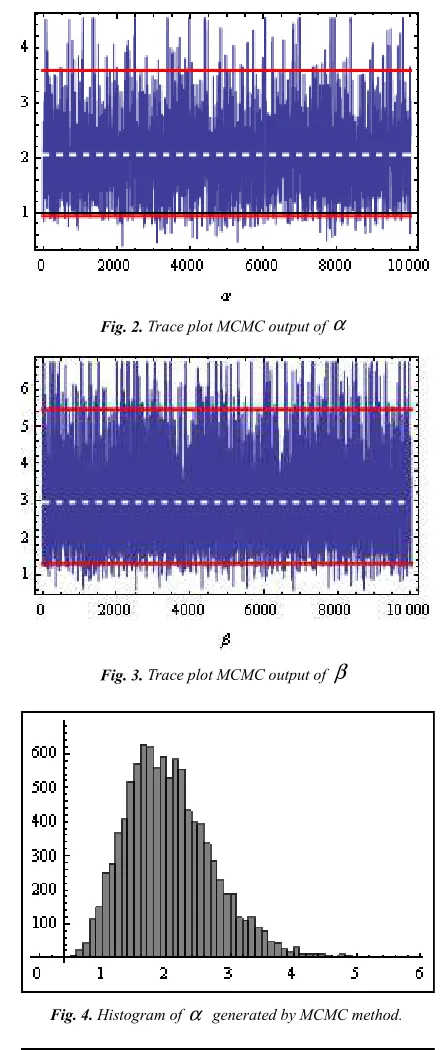
as given in (32) is plotted in Figure 1. It can be approximated by normal distribution function as mentioned in Subsection 4.1. Also the 95% , approximate maximum likelihood estimation (AMLE) confidence intervals, Bootstrap confidence intervals and approximate credible intervals based on the MCMC samples, the results are given in Table 1. Figures 2 and 3 plot the MCMC output of α and

β

, using 10000 MCMC samples (dashed line represent means and red lines represent lower and upper bounds of 95% probability intervals.). The plot of histogram of α and

β

generated by MCMC method are given in Figures 4 and 5. This was done with 1000 bootstrap sample and 10000 MCMC sample and discard the first 1000 values as `burn-in'.

Fig. 1. Posterior density function of α given

β

Fig. 2. Trace plot MCMC output of α

Fig. 3. Trace plot MCMC output of

β

Fig. 4. Histogram of α generated by MCMC method.

Table 1. Results obtained by MLE, Bootstrap and MCMC method of α and

.

β

Method Parameter Point Interval Length

MLEs α_β 2.1741 [-0.0166,4.3649] 4.3815 3.1153 [-0.5861,6.8168] 7.4029

Boot-p α_β 2.0938 [0.1518,3.9557] 3.8039 2.9777 [0.6380,5.9440] 5.3060

Boot-t α_β 2.1810 _3.1162 [0.1831,3.6436] _{[0.0744,5.0567]} 3.4605 _4.9823

MCMC α_β 2.0563 _2.9667 [0.9442,3.5859] _{[1.3008,5.4599]} 2.6417 _4.1591

6. Simulation Study

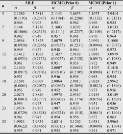
Table 2. Average values of the different estimators, the corresponding MSEs and coverage percentages when ( , )α β =(2, 3).

n _α MLE _β MCMC(Prior 0) _{α β} MCMC(Prior 1) _{α β}

5 2.1289 3.2814 2.1143 3.0633 2.1075 2.9414 (0.1193) (0.2347) (0.1184) (0.2286) (0.1132) (0.2131) 0.945 0.965 0.951 0.962 0.969 0.953 7 2.148 3.1736 2.1603 3.0202 2.1043 3.0133

(0.1066) (0.2315) (0.1111) (0.2237) (0.1109) (0.2117) 0.942 0.949 0.957 0.961 0.970 0.964 9 2.0544 3.2825 2.0079 3.0711 2.0991 3.1000

(0.0928) (0.2246) (0.0955) (0.2231) (0.0946) (0.2037) 0.949 0.957 0.948 0.964 0.955 0.973 12 2.1412 3.1068 2.1427 2.9168 2.0885 3.0979

(0.0921) (0.2132) (0.0922) (0.2128) (0.0912) (0.1988) 0.961 0.964 0.951 0.958 0.972 0.949 15 2.1410 3.0482 2.0007 3.06632 2.1707 3.1410

(0.0917) (0.2103) (0.0910) (0.2105) (0.0908) (0.1953) 0.951 0.963 0.946 0.958 0.963 0.954 18 2.1581 3.0609 2.0864 2.9813 2.0829 2.9962

(0.0861) (0.2057) (0.0862) (0.2054) (0.0812) (0.1806) 0.953 0.949 0.952 0.961 0.973 0.956 20 2.0271 2.8826 1.9975 2.9367 2.0135 3.0149

(0.0807) (0.1777) (0.0808) (0.1774) (0.0756) (0.1569) 0.954 0.943 0.947 0.949 0.951 0.956 23 1.9574 3.0367 1.9871 3.0279 1.9514 2.9829

(0.0729) (0.1528) (0.0721) (0.1518) (0.0613) (0.1404) 0.961 0.943 0.954 0.956 0.972 0.963 25 1.9924 2.9654 2.0214 3.1202 2.0581 2.9965

(0.0622) (0.1465) (0.0615) (0.1466) (0.0498) (0.1304) 0.955 0.961 0.953 0.958 0.941 0.971 Note: The first figure represents the average estimates, with the corresponding MSEs and coverage percentages reported below it in parentheses.

In order to evaluate the behavior of the proposed methods, Monte Carlo simulations were performed utilizing 1000 lower record samples from exponentiated Weibull distribution (EWD) for each simulation. The mean square error (MSE) is used to compare the estimators. The samples were generated by using ( , )

α β

=

( )

2,3 ,

(

1.5, 4

)

, with different sample of sizes ( )n . For computing Bayes estimators, we used the non-informative gamma priors for both the parameters, that is, when the hyper-parameters are 0 . We call it prior 0: a= = = =b c d 0. Note that as the hyper-parameters go to 0, the prior density becomes inversely proportional to its argument and also becomes improper. This density is commonly used as an improper prior for parameters in the range of 0 to infinity, and this prior is not

specifically related to the gamma density. For computing Bayes estimators, other than prior 0, we also used informative prior, including prior 1, a=1, b=1, c=2 and

1

d = , also we used the squared error loss (SEL) function to compute the Bayes estimates.

We also computed the Bayes estimates and 95% credible intervals based on 10 000 MCMC samples and discard the first 1000 values as `burn-in'. We report the average Bayes estimates, mean squared errors ( MSEs ) and coverage percentages. For comparison purposes, we also computed the MLEs and the 95% confidence intervals based on the observed Fisher information matrix. Finally, we used the same 1000 replicates to compute different estimates Tables 2 and 3 report the results based on MLEs and the Bayes estimators (using MCMC technique) using informative prior on both α and

β

.

Table 3. Average values of the different estimators, the corresponding MSEs and coverage percentages when ( , )α β =(1.5, 4).

n MLE MCMC(Prior 0) MCMC(Prior 1)

α β α β α β

5 1.6317 3.8784 1.4719 3.9650 1.4339 4.0668 (0.0852) (0.2604) (0.0867) (0.2659) (0.0708) (0.2345) 0.962 0.958 0.941 0.953 0.961 0.955 7 1.5757 4.1241 1.4952 3.9759 1.7371 4.1880

(0.0849) (0.2491) (0.0842) (0.2427) (0.0662) (0.2287) 0.958 0.941 0.953 0.971 0.942 0.959 9 1.5245 3.8819 1.4981 3.9705 1.3914 3.7998

(0.0789) (0.2309) (0.0770) (0.2302) (0.0649) (0.2181) 0.941 0.966 0.954 0.964 0.950 0.975 12 1.4083 3.9512 1.5127 3.8733 1.4447 3.8999

(0.0517) (0.2177) (0.0519) (0.2161) (0.0507) (0.1904) 0.964 0.956 0.967 0.950 0.967 0.956 15 1.4263 4.1285 1.4286 4.023 1.5075 3.9815

(0.0444) (0.1836) (0.0423) (0.1820) (0.0412) (0.1751) 0.954 0.957 0.951 0.958 0.963 0.961 18 1.6061 4.0660 1.6476 4.0798 1.5417 4.0634

(0.0373) (0.1532) (0.0378) (0.1597) (0.0326) (0.1394) 0.956 0.941 0.946 0.953 0.958 0.970 20 1.3995 3.9371 1.5554 3.8954 1.6709 3.8847

(0.0319) (0.1303) (0.0320) (0.1302) (0.0279) (0.1238) 0.959 0.952 0.959 0.949 0.956 0.963 23 1.7735 3.9715 1.737 4.125 1.5764 3.9278

(0.0308) (0.1293) (0.0302) (0.1256) (0.0197) (0.1168) 0.964 0.954 0.957 0.952 0.961 0.966 25 1.6240 3.9845 1.4875 4.0972 1.5278 3.9641

(0.0231) (0.1098) (0.0234) (0.1108) (0.0165) (0.0922) 0.949 0.962 0.955 0.959 0.961 0.959 Note: The first figure represents the average estimates with the corresponding MSEs and coverage percentages reported below it in parentheses.

7. Conclusion

technique to generate posterior sample. we observe the following:

From the results obtained in Tables 2 and 3. It can be seen that the performance of the Bayes estimators with respect to the non-informative prior (prior 0) is quite close to that of the MLEs.

Tables 2 and 4 report the results based on non-informative prior (prior 0) and non-informative prior, (prior 1) also in these case the results based on using the Gibbs sampling procedure are quite similar in nature when comparing the Bayes estimators based on informative prior clearly shows that the Bayes estimators based on prior 1 perform better than the MLEs, in terms of MSEs. From Tables 2-3, it is clear that the Bayes estimators based on informative prior perform more better than non-informative prior and the MLEs in terms of MSEs.

References

[1] Arnold, B. C., 1983. Pareto distributions. In: Statistical Distributions i Scientific Work, International Co-operative Publishing House, Burtonsville, MD.

[2] Arnold, B. C., Balakrishnan, N. & Nagaraja, H. N.,1998. Records, Wiley, New York.

[3] Resnick, S. I., 1987. Extreme values, regular variation, and point processes, Springer-Verlag,New York.

[4] Raqab, M. Z. & Ahsanulla, M., 2001. Estimation of the location and scale parameters of the generalized exponential distribution based on order Statistics. Journal of Statistical Computation & Simulation, 69: 109- 124.

[5] Nagaraja, H. N., 1988. Record values and related statistics-a review. Communication in Statistics Theory & Methods,17: 2223-2238.

[6] Ahsanullah, M., 1993. On the record values from univariate distributions, National Institute of Standards and Technology Journal of Research, Special Publications, 12: 1-6.

[7] Ahsanullah, M., 1995. Introduction to record statistics, NOVA Science Publishers Inc., Hunting ton, New York.

[8] Raqab, M. Z., 2002. Inferences for generalized exponential distribution based on record Statistics. Journal of Statistical Planning &Inference, 52: 339-350.

[9] Abd Ellah, A. H., 2011. Bayesian one sample prediction bounds for the Lomax distribution. Indian Journal of Pure and Applied Mathematics, 42: 335-356.

[10] Abd Ellah, A. H., 2006. Comparison of estimates using record statistics from Lomax model: Bayesian and non Bayesian approaches. Journal of Statistical Research and Training Center, 3: 139-158.

[11] Sultan, K. S. & Balakrishnan, N., 1999. Higher order moments of record values from Rayleigh and Weibull distributions and Edgeworth approximate inference, Journal of Applied Statistical Science, 9: 193-209.

[12] Preda, V. & Panaitescu, E., 2010. Constantinescu and S. Sudradjat, Estimations and predictions using record statistics from the modified Weibull model, WSEAS Transaction on Mathematics, 9: 427-437.

[13] Mahmoud, M. A. W., Soliman, A. A., Abd Ellah, A. H. & EL-Sagheer, R. M., 2013. Markov chain Monte Carlo to study the estimation of the coefficient of variation. International Journal of Computer Applications, 77: 31-37.

[14] Mudholkar, G. S. & Srivastava, D. K., 1995. The exponentiated Weibull family: a reanalysis of the bus-motor-failure data. Technometrics, 37(4): 436-445.

[15] Efron, B., 1982. The bootstrap and other resampling plans, In: CBMS-NSF Regional Conference Seriesin Applied Mathematics, SIAM, Philadelphia, PA, 1982.

[16] Hall, P., 1988. Theoretical comparison of bootstrap confidence intervals. Annals in Statistics, 16: 927-953.

[17] Geman, S. & Geman, D., 1984. Stochastic relaxation, Gibbs distributions and the Bayesian restoration of images. IEE Transaction on Pattern Analysis and Machine Intelligent, 12: 609-628.

[18] Smith, A. & Roberrs, G., 1993. Bayesian computation via the Gibbs sampler and related Markov chain Monte Carlo methods, Journal of Reliability & Statistical Society, 55: 3-23. [19] Metropolis, N., Rosenbluth, A. W., Rosenbluth, M. N., Teller,

A.H. & Teller, E., 1953. Equations of state calculations by fast computing machine. Journal of Chemistry Physics, 21: 1087-1092.

[20] Hastings, W. K., 1970. Monte Carlo sampling methods using Markov chains and their applications. Biometrika,57: 97-101. [21] Robert, C. P. & Casella, G., 2004. Monte Carlo statistical

methods, second edition, Springer, New York.