Download Download PDF

FINITE ELEMENT MODELLING OF STEEL POLES FOR POWER

PRODUCTION AND TRANSMISSIONS

M. Aliyu

_{and O. S. Abejide}

1, 2,

_D

_C

_E

_,

_A

_B

_U

_,

_Z

_,

_K

_S

_.

_NIGERIA

E-mail addresses:

_{[email protected]}

_,

_{[email protected]}

ABSTRACT

Materials used in civil engineering constructions display wide range in their engineering properties; a structural engineer is required to quantify the risks and advantages of using such materials. Continuous supply of electricity is essential for every nation and electric poles are been susceptible to extreme damages caused by natural hazards such as snow, wind, ice, earthquake etc. These actions can knock down poles thereby causing damage and disruption of power supply. Selecting a pole material such as steel for power transmissions will sufficiently help in distributing power due to its superior material properties. The determination of the response of the steel poles to loads is accomplished by the aid of Finite Element (FE) coded in software, ABAQUS CAE. The extent of damage as a result of deflections as per stresses and displacements were effectively measured and simulated in the software. The result in ABAQUS shows that the steel poles will not suffer any reasonable deformation when loaded indicating that steel poles material properties are sufficient to provide adequate resistance against actions such as deformations and deflections during their service lives.

Keywords: Steel poles, Deformation, Finite Element, ABAQUS.

1. INTRODUCTION

Electric transmission poles are unique structures that are used to support conductors and shield wires of a transmission line; they are either lattice type or pole type structures. Lattice type structures are used for the highest of voltages while poles types are used for low to medium tension. Materials used in power pole construction can be wood, reinforced concrete, steel or even composite material poles, such as FRP poles that are becoming more prevalent nowadays [1]. Steel poles hold up wires that bring electricity and other modern amenities to our homes. These poles help provide for the growing network of telephones, televisions, computers and satellite gadgets.

In the event of natural disasters, the continuous supply of electricity is essential for the welfare, economy, and security of our societies. Steel poles are by far the strongest material used in power pole construction, but require less maintenance than the other varieties. Consequently, steel poles are of great significance [2].

In recent years, utility companies have been searching for cost-effective alternatives to timber poles and other pole materials due to environmental concerns, high cost of maintenance, and need for improved aesthetics. In North America for example, steel poles usage has more than tripled, as reported among the estimated 185 million electric distribution poles that crisscross the United States and Canada; 600 utilities use steel pole alternative [3].

An electric steel pole which is part of transmission lines or distribution system acts as a cantilevered structure, which is designed and analyzed as a tapered member with combined axial and bending loads. The forces acting on the poles are from the vertical loading (comprising dead weight of conductors, cross arms, insulators) and the horizontal loading due to wind pressure on conductors and pole [4].

The overall sustainable economic growth, productivity, and the well-being of a nation depend heavily on the functionality, reliability and durability of its constructed facilities, it is for this reason that the strength of these

Vol. 38, No. 4, October 2019, pp.

840 – 847

Copyright© Faculty of Engineering, University of Nigeria, Nsukka, Print ISSN: 0331-8443, Electronic ISSN: 2467-8821

steel poles in service need to be assessed in a stochastic manner, while accounting for all the parameters associated with their performance in service during their design life.

2. CONCEPT OF POWER SYSTEM

Electricity plays an important role in the socio-economic and technological development of every nation, traditionally; power system is one of the instruments used for converting and transporting power to meet various demands. The main function of the power system is to convert energy from one form to another and distribute it to the consumers. The electric power system has three main components that can be broadly divided into three subsystems, and they are: generation, transmission, and distribution [5].

The generation aspect deals mostly with the source of power, ideally with specified voltage and frequency. For example, the voltage levels for transmission system ranges from 34.5 kV to as high as 1100 kV in the United States of America [6]. The transmission is usually the link between the generating station and the distribution system in terms of voltage levels. It transports the power in bulk using the transmission systems that use wires supported by steel towers that are about 45m high and spaced about 240m apart [7]. In other words, the transmission system is part of the system between transmission and the consumer service point [8]. The distribution component deals with the distribution of electricity at lower voltages for our daily consumption via poles. Poles are of two genres; first the utility poles which are grouped into two kinds; utility transmission and utility distribution and the second genre includes poles for lightening, traffic and even for intelligent traffic structures. Both genres of poles are analyzed and designed by the same structural principles, but they differ in governing codes and industry practice [9].

2.1 Material of Poles

Poles are supporting structures which carry the overhead conductor. They are of different types; they could be of wood, concrete, steel, or even composite material. This study focuses on steel distribution poles. The use of steel poles has become the product of choice because of its construction efficiency and the use of these poles is just beginning to make in-roads in distribution lines. The steel distribution pole is an engineered product, each designed to meet specific strength and load requirements. The strength of these

steel poles is based on the minimum values of ultimate tensile strength of steel. They are tested and fabricated under several code specifications such as the American Society of Civil Engineers (ASCE) tolerance [10]., National Electricity Safety Code (NESC) [11]., Indian Standard (I.S) specification for tubular steel poles for overhead power lines load requirements [12].

2.2Structural Loadings of Steel Poles

Pole design is usually dependent on the power and voltage that is to be transmitted; the design is based on the principle of conductor loading. Steel poles are sometimes specified in situations where poles of high strength are required. Stress imposed on poles are calculated as if they were a cantilever beam fixed at one end; also ground line moments, as well as cross-arms, if attached, must be designed to withstand the load of conductor and equipment.. Also the need to know how to calculate cross-arm and insulator loads, these values with proper factors of safety (intended to account for all forms of uncertainty, including material property variability) applied are used in the selection of the pole loads. Most of the forces on a pole are from the vertical loading comprising dead weight of conductors, cross-arms, insulators and associated hardware, the horizontal loading due to wind pressure on conductors and pole [4].

Figure 1: Steel Distribution Pole Layout [12].

Where; 𝐴 − 𝐴 = line of application of resultant of wind loads on wires and pole;𝐻 = overall height above ground in m;𝑙1, 𝑙2, 𝑎𝑛𝑑 𝑙3 = Distance in m from A-A to bottom of each

section (in case of bottom section, it is up to GL only);𝐷1𝐷2𝐷3=

Outside diameter of top, middle and bottom sections of pole, p = Wind pressure on flat surface 𝑁/𝑚2_{;ℎ = height of conductors on}

cross-arm from GL;𝑛 = Number of conductors;𝑑 = diameter of conductors; 𝑠 = Sum of half the spans on each side of pole;𝑃1=

equivalent wind load on pole, calculated as acting at A-A; 𝑃2=equivalent wind load on conductor calculated as acting at

A-A;𝑃 =total wind load as acting at A-A;𝑃 = 𝑃1+ 𝑃2 in N;𝐺𝐿 =

ground level;𝐵𝑀 = bending moment.

2.3 Wind Load

The principal wind loadings on poles can be grouped into two categories; wind loading concentrated along the height of the pole and wind loading concentrated at the level of the cables usually 0.3m from the tip of the pole. The load on the wires is calculated by multiplying the wind pressure by the diameter of each wire, by the length of the span and the result by 2/3 to allow for circular section. Then the equivalent load acting at A-A can be calculated as follows:

Wind load on conductors =𝑃𝑛𝑠𝑑ℎ

100 × 2

3 𝑁, acting at h meters from GL

BM due to wind load at GL =𝑃𝑛𝑠𝑑ℎ

100 × 2 3 𝑁. 𝑚.

Equivalent load acting at A-A =𝑃𝑛𝑠𝑑ℎ

100𝑙3 ×

2 3 𝑁 Therefore,

𝑃2=

𝑃𝑛𝑠𝑑ℎ 150𝑙3

𝑁 (1)

The wind load on pole is next calculated and expressed as the equivalent load acting at the same point as the load imposed by wires.

Wind load on pole

=2𝑃𝐷1

300 [𝐻 − (𝑙3− 𝑙1)] (2)

Acting at a distance of,

𝐻 −𝐻 − (𝑙3− 𝑙1)

2 +

2𝑃𝐷2(𝑙3− 𝑙1)

300 +

2𝑃𝐷3(𝑙3− 𝑙2)

300 (3)

Where: 𝐻 −𝐻−(𝑙3−𝑙1)

2 is from G.L,

2𝑃𝐷2(𝑙3−𝑙1)

300 acting at a distance [(𝑙3− 𝑙2) +

𝑙2−𝑙1

2 ] from G.L and

2𝑃𝐷3(𝑙3−𝑙2)

300 is acting at a distance 𝑙3−𝑙2

2 from GL.

Therefore, Bending Moment at ground line is given as:

𝐵𝑀 = 2𝜌

300[𝐷1{𝐻 − (𝑙3− 𝑙1)} {𝐻 −

𝐻 − (𝑙3− 𝑙1)

2 }

+ 𝐷2(𝑙2− 𝑙1) (𝑙3−

𝑙1

2− 𝑙2

2)

+ 𝐷3(𝐿3− 𝐿2)

𝑙3− 𝑙2

2 ] (4)

Say 𝐵𝑀 = 𝑊𝑀,

Equivalent load acting at A-A

𝑃1=

𝑊𝑀 𝐿3

(5)

So that total load:

𝑃 = 𝑃1+ 𝑃2 (6) The methodology applied for the evaluation of the assumed behavior of the steel pole due to its applied loads and strength using Finite Element Analysis coded in ABAQUS/CAE for power production and transmission is given in the following section.

3. METHODOLOGY

3.1 Probabilistic Testing using FEA Coded in ABAQUS Software

ABAQUS/CAE is a general-purpose FEM program. The aim is to analyse how reliable or otherwise the failure regions in the pole structure are. ABAQUS adopts techniques for evaluating failure regions and stresses.

3.2 Finite Element Analyses and Modelling Applied to Steel Poles

The use of Finite Element Method (FEM) has gained abundant popularity in recent years due to advances in high-speed computers. Finite Element Analysis (FEA) is a numerical method for solving problems of engineering and mathematical physics. These

G.L

methods originated from the need for solving complex structural analysis problems in civil and aeronautical engineering. The objective of analysis using ABAQUS finite elements programming is to examine the assumed behavior of a steel pole due to its applied loads. Consequently, the stresses and deformations of the pole under various load effects will be determined. In addition, it is an important procedure to figure material properties as they appear in the target structure.

The extent of failure, stresses and displacements is effectively measured with the aid of finite element (FE) which is simulated in ABAQUS software. The FEM helps tremendously in producing stiffness and strength visualizations and also in minimizing weight, materials, and costs. The calculation is then determined using the results obtained from ABAQUS finite element programming. A Finite Element Analysis (FEA) program would be used to validate the strength of the pole. If the pole were too weak, it would not hold up under the stress of the attached wires, if it were over designed, its lifecycle would require more energy [14]. Table 1 indicates the parameters used in the FE modeling in ABAQUS.

3.3 Mathematical formulations of Finite Element (FE)

Finite Element method is a special form of the well-known Galerkin and Rayleigh-Ritz methods of finding approximate solution of differential equations. In both methods the governing differential equation first is converted into an equivalent integral form. The Rayleigh-Ritz method employs calculus of variations to define an equivalent variation while the Galerkin method uses a more direct approach. An approximate solution, with one or more unknown parameters, is chosen, but in general, this assumed solution will not satisfy the differential equation. The integral form represents the residual obtained by integrating the error over the solution domain. Employing a criterion adopted to minimize the residual gives equations for finding the unknown parameters. For most practical problems, solutions of differential equations are required to satisfy not only the differential equation but also the specified boundary conditions at one or more points along the boundary of the solution domain. In both methods some of the boundary conditions must be satisfied explicitly by the assumed solutions, while others are satisfied implicitly through the minimization process. The boundary conditions are

thus divided into two categories; essential and natural. The essential boundary conditions are those that must explicitly be satisfied, while the natural boundary conditions are incorporated into the integral formulation. In general, therefore, the approximate solution will not satisfy the natural boundary conditions exactly.

In a method known as the least–squares weighted residual method the error term is squared to define error as follows:

𝑒𝑇 = ∫ 𝑒2 𝑥1

𝑥0

𝑑𝑥 (7)

The necessary conditions for the minimum of the total squared error give n equations that can be solved for unknown parameters:

𝜕𝑒𝑇

𝜕𝑎𝑖

= 2 ∫ 𝑒 𝜕𝑒 𝜕𝑎𝑖 𝑥1

𝑥0

𝑑𝑥 = 0; 𝑖 = 0,1, …. (8)

Thus in the least-squares method the weighting functions are the partial derivatives of the error term e(x)

Least-squares weighting functions:

(𝑋) = 𝜕𝑒 𝜕𝑎𝑖

; 𝑖 = 0,1, … . 𝑛 (9)

A more popular method in the finite element applications is the Galerkin method. In this method, instead of taking partial derivatives of the error function, the weighting functions are defined as the partial derivatives of the assumed solution.

Galerkin weighting functions:

𝑊𝑖 (𝑋) =

𝜕𝑢

𝜕𝑎𝑖

; 𝑖 = 0,1, … . 𝑛 (10)

Thus the Galerkin weighted residual method defines the following n equations to solve for the unknown parameters:

∫ 𝑒 𝜕𝑢 𝜕𝑎𝑖 𝑥1

𝑥0

𝑑𝑥 = 0; 𝑖 = 0,1, … (11)

It turns out that for a large number of engineering applications the Galerkin method gives the same solution as another popular method, the Rayleigh-Ritz method. Furthermore, since the least –squares method has no particular advantages over the Galerkin method for the kinds of problems we encounter; only the Galekin method is presented in detail. So far in developing the residual we have considered error in satisfying the differential equation alone. A solution must also satisfy boundary conditions. In order to be able to introduce the boundary conditions into the

weighted residual, we use mathematical

Table 1: Input Parameters for Finite Element Analysis (FEA) Material Yield Strength

(N/mm2₎

Young Modulus (N/mm2₎

Density

(Kg/m3₎ Poisson’s ratio Thermal Coefficient

Steel 500 209E+03 7850 0.3 12 × 10−6_per o_C

The integration-by-parts formula is used to rewrite an integral of a product of a derivative of a function, say f(x), and another function, say g(x), as follows:

∫ [𝑑 𝑑𝑥

𝑥1

𝑥0

(𝑓(𝑥))] 𝑔(𝑥)𝑑𝑥

= 𝑓(𝑋1)𝑔(𝑋1) − 𝑓(𝑋0)𝑔(𝑋0)

− ∫ [𝑑 𝑑𝑥

𝑥1

𝑥0

(𝑔(𝑥))]𝑓(𝑥)𝑑𝑥 (12)

Below is a summary of the steps involved in running the ABAQUS software for steel pole-modeling.

(a) Part module: this module provides the tools for creating, editing and managing the elements of the steel pole. Its features capture the design intent and geometry information of all of the elements listed above.

(b) Property module: this module specifies the different characters and material properties of the elements created in the part module. The table 1 gives the summary of parameters used in the part module session.

(c) Assembly module: the element parts of the modeled are assembled in this module.

(d) Step module: this module is used to create the analysis type and sequence. Specifying the sequence provides a convenient way to capture changes in the loading and boundary conditions of the model.

(e) Load module: this module is also step dependent. The boundary conditions and load types are specified. For this study, the steel pole is fixed at the bottom and free at the top where the load is acting.

(f) Job module: this module helps to the job and submits it for analysis while you monitor its progress.

(g) Visualization module: this module provides the graphical display of structural mechanics and the finite element results of the model. It obtains its result from the output data.

4. RESULTS AND DISCUSSION 4.1 Results

The steel pole result output are generated based on the design input from the ABAQUS design environment, the model of the steel poles is given as shown in Plates I – IV and figures 1 to 2. The analysis of the poles following a non-linear stress pattern and deformations are discussed further. The loads acting on pole comprise of wind loads concentrated along the height of the poles, wind loads concentrated at the level of the cables usually 0.3m from the tip of the pole and dead loads which comprises self-weight of aluminium, street lamp on the pole, cross arms and pin connection attached and of course self-weight of steel, For the purpose of this study, the typical pole was subjected to load of 20kNfor 7, 8, 9, 10 and 12m height of poles; the boundary conditions for the steel poles are fixed at one end and analyzed just as a cantilever beam with the load acting at its free end. The results presented here are, the maximum principal stresses and von Mises stresses on the poles, as in the plates and figures.

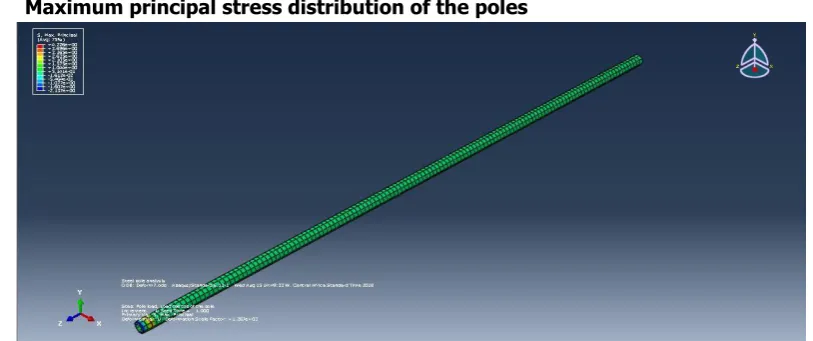
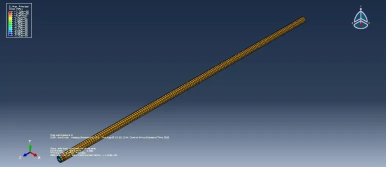
(i.) Maximum principal stress distribution of the poles

Plate II: Maximum principal stress for the pole (9m)

Figure 2: Relationship of maximum values of Principal stress (tension) to different pole lengths

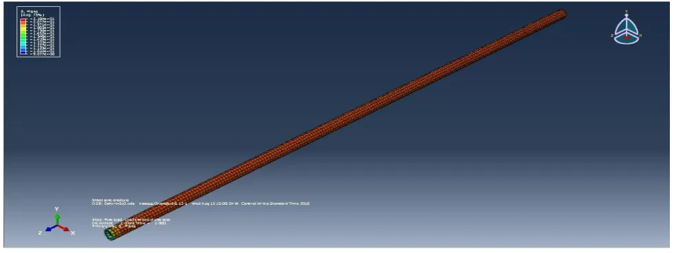
(i.) Von Mises maximum stress distribution for the pole

The Plate III shows the stress distribution for the 9m height poles while that of 10m high poles is shown in Plate IV.

Plate III: Von Mises stress for the steel pole (9m)

0.00E+00 2.00E-03 4.00E-03 6.00E-03 8.00E-03 1.00E-02

7 8 9 10 12

M

ax.

Pr

in

ci

p

al

S

tr

e

ss (N

/m

m

2)

Plate IV: Von Mises stress for the steel pole (10m)

Also, Figure 3 indicates the relationship of maximum values of von mises stress to different pole length.

Figure 3: Relationship of maximum values of Von-Mises stress to different pole lengths

The steel poles in service did not suffer any stress deformation failure due to the stiffness of the material property; the non-linear finite element stress analysis considering a linear perturbation step perpendicular load yielded a deformation scale factor of 1.00E0 resulting into a maximum principal stress value of 2.322E-03𝑁 𝑚𝑚⁄ 2and maximum stress value of

9.077E-03𝑁 𝑚𝑚⁄ 2.

The von mises stress pattern obtained after the analyses of the typical pole can also be seen in Figure 3 above. The Finite element stress analysis considering a linear perturbation step perpendicular load yielded a deformation scale factor of 1.00E0, resulting to a von Mises minimum stress values of 2.183E-01𝑁 𝑚𝑚_⁄ 2 _and maximum stress value of 8.34E-03𝑁 𝑚𝑚_⁄ 2_{.The reddish} yellow colors observed at the bottom of the steel poles indicate where the maximum values of von Mises stresses are, however, for all the lengths of the poles considered, the poles did not show any noticeable deformations after the analyses in the software and, hence, it is an indication that the pole will be

applied loads. The maximum values of the results obtained are usually computational tools which aid designers in showing how the structure will behave when loaded in order to mitigate actions such as severe winds, deformations and total collapse.

5. CONCLUSIONS

From the results obtained in the previous section, Finite Element Analysis software ABAQUS CAE can be adopted for the static analyses of the poles and this method can be used to simulate the behavior of the steel poles. The extent of damage as a result of deflections as per stresses and displacements were effectively measured; values of principal stresses and von mises as well as their places of maximum and minimum values were obtained, which are far below the yield stress of the steel pole. The choice of material to be used is based on several factors such as available resources and functional requirements, but steel poles provide better performance than other types of poles. However, Finite element analyses coded in ABAQUS and other computer based analytical packages can be 0.00E+00

2.00E-03 4.00E-03 6.00E-03 8.00E-03 1.00E-02

7 8 9 10 12

Vo

n

m

ises

(N

/m

m

2)

used to enhance studies on power distribution poles. Also, the design of a structure to provide a known level of reliability requires that a reliability-based design methodology be established especially for steel poles before construction is carried out. The steel poles are safe throughout their design life and even beyond since the stresses developed in them due to the applied load are low. This will justify structural safety and economy and with minimal maintenance.

6. REFRENCES

[1] Oyejide, S. A., Adejumobi, I. A., Wara, S. T. and Ajisegiri, E. S. A. Development of a Grid-Based Rural Electrification Design: A Case Study of Ishashi and Ilogbo Communities in Lagos State. Journal of Electrical and Electronics Engineering IOSR-JEEE. e-ISSN: 2278-1676,www.iosrjournals.org. Vol. 9, 2014, pp. 12-21.

[2] Kenney, I. Types of Power Poles. Retrieved from

www.livestrong.com/article/138585. On

September 11, 2017.

[3] Lacoursiere, B. Steel Utility Poles: Advantages and Applications. Paper Presented at The Rural Electric

Power Conference.

doi.org/10.1109/repcon.1999.768681.

[4] Oritola, S. F. Improvement of Production Method for Electric Transmission Concrete Pole in a Developing Zone in Nigeria. Assumption University Journal of Technology. Vol. 9, 2006, pp. 267-271. [5] William, E. Standard Specifications for Wood Poles.

Paper Presented at the Utility Pole Structures

Conference and Trade Show; Reno/Sparks, Nevada, Vol. 1, 2005, pp. 6-7.

[6] Brown, R. E. Electric Power Distribution Reliability: CRC press, 2008.

[7] Willis, L., and Philipson, L. Understanding Electric Utilities and De-regulation. Steel Market and Development Institute. SMDI, Vol. 27, 2005. [8] Pabla, A. S. Electric Power Distribution, Tata

McGraw-Hill Publishing Company Limited, (5th Edition), New Delhi, India, 2008.

[9] Crosby, A. Special Research Topic Report on Current Practice in Utility Distribution Poles and Light Poles, 2011.

[10]ASCE. American Society of Civil Engineers. Design of Steel Transmission Pole Structures. ASCE Manual No. 72. American Society of Civil Engineers, New York, 2001.

[11]NESC. National Electric Safety Code C2-2007. New-York: Institute of Electrical and Electronics Engineers, Inc, 2002.

[12]Indian Standard IS 2713. Specification for Tubular Steel Poles for Overhead Power Lines, Second Revision, 2002.

[13]Barone, G., and Frangopol, D. M. Reliability, Risk and Lifetime Distributions as Performance Indicators for Life-Cycle Maintenance of Deteriorating Structures. Reliab Eng Syst Saf; Vol. 123, 2014, pp. 21–37.