Estimation of electrical conductivity of a soil solution from the monitored TDR data
and an extracted soil solution
Katsutoshi Seki1*, Teruhiko Miyamoto2, and Yukiyoshi Iwata2 1Natural Science Laboratory, Toyo University, 5-28-20 Hakusan, Tokyo 112-8606, Japan
2Agricultural Environment Engineering Research Division, Institute for Rural Engineering, NARO, 2-1-6 Kannondai, Tsukuba, Ibaraki 305-8609, Japan
Received April 24, 2018; accepted November 4, 2018
*Corresponding author e-mail: [email protected] © 2019 Institute of Agrophysics, Polish Academy of Sciences A b s t r a c t.In order to establish sustainable agricultural
prac-tices and to avoid excess fertiliser application, it appears important to understand the process of water and solute transport. With a view to analysing transport through the soil, based on the data obtained by means of time domain reflectometry, the relationship between the volumetric water content, the apparent electrical conducti- vity, and the soil solution electrical conductivity should be known. This paper proposes a new method for estimating the three para- metersrelationship by optimising the parameters obtained through Rhoades model with the Levenberg-Marquardt method. The pro-posed method systematically determines the initial parameter set required to conduct nonlinear optimisation. The method was used to estimate the continuous apparent electrical conductivity data based on the time domain reflectometry dataset, obtained from the field and occasional measurement of soil solution electri-cal conductivity data of the soil water, which was extracted by means of a suction sampler installed in the field. Compared with the conventional method where the parameters of Rhoades model are calibrated with a 2-step linear regression by means of labora-tory experiment, the soil solution electrical conductivity estimated with the proposed method was closer to the field data, yielding smaller root mean square error values. Supplementary use of the dataset obtained through a laboratory experiment under dry and wet conditions improved the accuracy of parameter estimation.
K e y w o r d s: time domain reflectometry, Rhodes model, para-meter estimation
INTRODUCTION
In order to establish sustainable agricultural practices and to avoid excess fertiliser application, it is important to understand the process of water and solute transport. Measuring the volumetric water content (θ) and the appa- rent soil electrical conductivity (ECa) under field conditions is generally required for this purpose. Time domain reflec
-tometry (TDR) is widely used for determining θ and ECa
simultaneously (Noborio, 2001). Moreover, multi-sensor probes have also been developed recently to assess θ and
ECa, with continuous and non-destructive measurements
(Scudiero et al., 2012; Vaz et al., 2013). By using these measurement techniques, we can easily obtain the θ and
ECa data in fields.
It does not appear practical to assess solute transport in soil using ECa under transient conditions because of the
strong dependence of ECa on θ. Therefore, ECa must be
related to the soil solution electrical conductivity (ECw) so
as to estimate the solution concentration under transient conditions with varying water content. The physico-empiri-cal and / or theoretiphysico-empiri-cal models describing the dependence of
ECa on ECw and θ (e.g. Rhoades et al., 1976; Rhoades et al.,
1989; Mualem and Friedman, 1991; Malicki and Walczak, 1999; Hilhorst, 2000) are used to estimate ECw for a given
combination of the measured ECa and θ in a particular soil
(Mallants et al., 1996; Risler et al., 1996; Das et al., 1999; Muñoz-Carpena et al., 2005; Miyamoto et al., 2015).
Laboratory calibration experiments are conducted using repacked soil columns to obtain model parameters for the
ECw − ECa − θ relationship (Heimovaara, 1995; De Neve et
al., 2000; Muñoz-Carpena et al., 2005; Wilczek et al., 2012; Miyamoto et al., 2015). However, this calibration method
is not suitable for field measurements because soils in the field are often structured and more naturally heterogeneous
than the uniformly repacked soil columns. Moreover, the calibration procedure of a 2-step linear regression requires that multiple datasets of precisely the same water content or the same electrical conductivity are obtained, which
proposed a field calibration procedure, which is an in situ
mass balance approach with a TDR probe installed vertical-ly on the soil surface. This calibration procedure, however, can be only applied to the top soil layer.
Sensor pairing is a field measurement method of the soil
water characteristic (Baumgartner et al., 1994). The paired sensors, such as neutron moisture meter access tubes or TDR probes, and tensiometers are often used to
simulta-neously determine θ and the matric potential (ψ). As a re- sult, the θ − ψ values are obtained. In an similar way, the simultaneous measurements of ECw−ECa−θ values, using
soil solution samplers and TDR probes, will also be a use-ful method for an in situ determination of the ECw− ECa− θ
relationship.
The objective of this study is to develop a method to identify the parameters of Rhodes model (Rhoades et al., 1976) for the ECw− ECa− θ relationship based on a dataset
of the ECw, ECa and θ values which are measured in the field. To this end, we have designed a calculation procedure
by adopting the Levenberg-Marquardt optimisation method (Marquardt, 1963), which has become a standard in
non-linear least-square fitting among both soil scientists and hydrologists (Šimůnek and Hopmans, 2002; Seki, 2007).
We have compared the ECw estimated from the proposed
method with the one obtained from the conventional meth-od of a 2-step linear regression, as shown by Miyamoto
et al. (2015). In addition, we have discussed a supplemen-tal use of the dataset of ECw, ECa and θ obtained through
a laboratory experiment to improve the accuracy of the pro-posed method.
MATERIALS AND METHODS
The field data published in Miyamoto et al. (2015) were
used in this study. The field experiment was carried out in the experimental field at the National Agriculture and Food
Research Organization in Tsukuba, Japan. The soil at that site was an Andosol (IUSS Working Group, 2014). The soil
profile was divided into two layers; the boundary between
the surface and subsurface layers (topsoil and subsoil) was at 0.5 m depth. The bulk densities of topsoil and subsoil were 710 and 630 kg m-3, respectively. Saturated
hydrau-lic conductivities of these soils were 35.0 and 30.0 mm s-1,
respectively. The soil water retention curves of topsoil and
subsoil are shown in Fig. 1. The field was fertilised with
20.0 g m-2 of N, 8.7 g m-2 of P and 16.6 g m-2 of K, used as
chemical fertilisers, on 25 December 2007. Theground sur-face was maintained in an unplanted condition throughout
the field experiment until 31 August 2008.
Dielectric permittivity of the soil (εa) and ECa were
meas-ured with TDR probes installed horizontally into pit faces at three locations and at three depths (0.2, 0.4, and 0.6 m, respectively) during the experimental period, in order
to detect the TDR waveforms reflected from the probes.
A cable tester (Tektronix, 1502B) was used to detect the
time domain of the electromagnetic wave, along with the probes. The observed data were recorded using a portable computer every hour. A copper-constantan thermocouple was installed in the central pit at each of the three depths to measure temperature in a continuous manner, which was
recorded by means of a datalogger (Campbell Scientific
Inc., CR10X) every hour. The relationship between εa and
θ was calibrated through a laboratory experiment, and the values of εa were converted into the respective values of
θ under field conditions, using the calibration equation.
The measured ECa values were calibrated to the value at
25°C with the temperature correction factor taken from Heimovaara et al. (1995).
The porous ceramic soil solution samplers were also buried at three depths. Two samplers were buried at each depth. The soil solution was sampled once to three times
a month by applying a suction of 50-70 kPa during the field
experiment. ECw was measured for each extracted soil
solu-tion using a portable EC meter (HORIBA ltd., Twin Cond). The average of 2 measured values obtained for each soil depth was used in the analysis. As a result, during 8 months of the measured period, 17 data points of ECw in the field
were obtained.
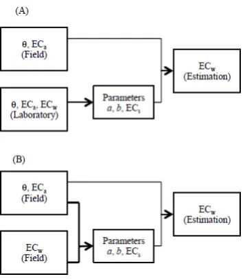
Figure 2A shows the process of estimating ECw by
means of the conventional method. Rhoades et al. (1976) derived the following equation:
ECa = ECwθT + ECs, (1)
where: T is the transmission coefficient which accounts for
the tortuous nature of the current lines and any decreases in the mobility of the ions near the solid-liquid and liquid-gas interfaces, and ECs is the surface conductivity via
exchangeable cations. They assumed that T is linear to θ, based on the empirical relationship by Gupta and Hanks (1972), which is as follows:
T = aθ + b, (2)
where: a and b are constants. Using the Eq. (2), the follow-ing equation was derived:
0 0.1 0.2 0.3 0.4 0.5 0.6 0.7 0.8
0.1 10 1000
Vol
um
et
ric
w
at
er c
ont
ent
,
q
Matric suction (kPa)
topsoil subsoil
ECa = (aθ+b) θECw + ECs. (3)
The conventional method is a 2-step linear regression. In
the first linear regression, for different sets of water content
(e.g., θ = 0.35, 0.40, 0.50, 0.60 for the experiment con-ducted by Miyamoto et al., 2015) the relationships between
ECw and ECa were written, and the fitted lines with slope
S = (aθ + b)θ and intersect ECs were obtained. In the second
linear regression, S/θ was plotted against θ, and the linear
fit yielded a and b. Finally, the Rhoades parameter set, a, b
and ECs was used to estimate ECw based on the measured
θ and ECa from Eq. (3). The conventional method requires
that multiple datasets of precisely the same water content
are plotted in the first regression to obtain parameters for
the second regression.
In the proposed method, the field-obtained values of θ,
ECa and ECw were basically used to determine a, b and ECs
of Rhoades model (Fig. 2B), with a successive optimisation technique as follows. In the present study, we used 17 ECw
data obtained from soil solution samplers. By coupling the data with the θ and ECa values measured with TDR probes in the field, both at the same depth and on the same day,
we obtained 17 sets of measured data (θ, ECa, ECw), which
were then used to estimate the parameter set (a, b, ECs).
Eq. (3) can be transformed as follows:
. (4)
Equation (4) shows the linear relationship between θ
and (ECa – ECs)/ECwθ. At first, ECs was assumed to be 0.25
dS m-1, one of the values obtained in Rhoades et al. (1976),
and the parameters a and b were obtained with the linear regression of equation (4). Then, a, b and ECs were
opti-mised with Eq. (3) simultaneously by the non-linear least square optimisation algorithm of Levenberg-Marquardt method (Marquardt, 1963).
Let the independent variable vector x in Eq. (3) be
defined by x= (x1, x2) = (θ, ECw), and the parameter
vec-tor pbe defined by p= (p1, p2, p3) = (a, b, ECs). The model
Eq. (3) is rewritten as:
f(x, p) = (p1x1+p2)x1x2 + p3. (5) Let the data points be denoted by:
(Yi, Xi) = (Yi, X1i, X2i), i = 1, 2, …, m, (6)
where: X1i, X2i, and Yi are the i-th data point of θ, ECw, and
ECa, respectively. The objective function of the least square
analysis O(p) is:
, (7)
where: the weights wi are normally set to 1 (unity). The
Levenberg-Marquardt algorithm efficiently solves
para-meter vector p so that O(p) is minimised. The Levenberg
-Marquardt method requires an initial estimate of parameter vector p. It then updates the estimate iteratively to find the final estimate of p. In the iterative procedure, vector p may not converge to a proper value when the initial estimate
of the parameter is not close enough to the final solution.
Therefore, selecting a reasonably good set of the initial parameter is a very important step for this algorithm. In the proposed method, the initial estimate of parameter vectorp
can be obtained systematically by the regression of Eq. (4) as described above.
The difference in the two methods shown in Fig. 2 con- cerns the methods of obtaining the Rhoades parameters (parameter vector p). The advantage of using the pro-posed method is that it does not require separate laboratory experiments that are both time-consuming and tedious. The conventional method requires calibration curves of the
ECw−ECa relationship for the same θ values. Such data are not usually available in the field, and thus the conventional
method can only be used with laboratory data. The pro-posed method does not require that the θ values be exactly
controlled, and thus the field data can be directly used for
obtaining Rhoades parameters. Moreover, as the conven-tional method simultaneously optimises all the parameters, it may require a smaller dataset for estimation. To verify whether the proposed method requires a smaller amount of data, we also performed calculation with smaller data-sets. From each month between January and August, one measuring dataset of (θ, ECa, ECw) was selected so that the
interval between the data points was around 30 days, and 8 data were used in the analysis.
The algorithm was implemented in the mathematics-oriented programming language of GNU Octave. The programme first fits the given dataset of θ, ECw and ECa
to Eq. (4) to get the initial estimate of the parameter set,
and then the initial parameter set is successively optimised with the iterative procedure of the Levenberg-Marquardt
method to get the final parameter set of a, b and ECs. In the
programme, the parameters were constrained with a > 0 and 0 < ECs< min (ECa).
RESULTS AND DISCUSSION
Table 1 shows the parameters used in Eq. (3) that were estimated on the basis of the ECw values of the extracted soil
solution, and θ and ECa were measured with TDR probes
using the developed method (Fig. 2B). Figure 3 shows the relationship between the measured and estimated ECa with
parameters in Table 1 of the 3 TDR probes at each depth. The agreement between the measured and estimated ECa
is not very good, compared to the laboratory calibration experiment outlined by Miyamoto et al. (2015), because
the field experiment could not be controlled to the same
extent as the laboratory experiment. However, many plots were found to be close to the identity line.
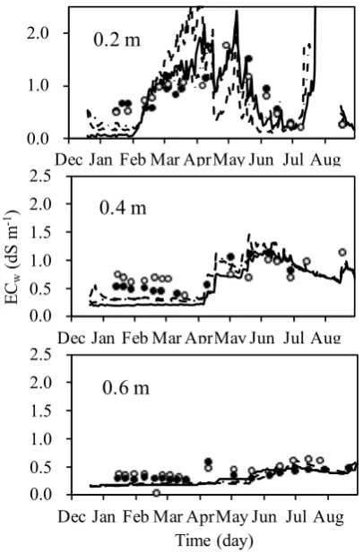
Figure 4 shows the change in the estimated ECw that
was calculated from the θ and ECa values measured with
TDR probes, and parameters in Table 1, compared with the
ECw directly measured from the soil solution. The
estima-tion at topsoil (0.2 m depth) was not successful because the
Table 1. Estimated parameters with field extracted soil solution and field measured TDR data
Depth 0.2 m 0.4 m 0.6 m
Probe ID 2A 2B 2C 4A 4B 4C 6A 6B 6C
a 3.7333 4.2508 5.1457 0.4019 0.3292 0.3689 0.0011 0.0000 0.0001
b -1.5934 -2.0348 -2.3268 0.5228 0.1762 0.1433 1.0683 1.0408 1.0429
ECs 0.0463 0.0182 0.0000 0.0000 0.0000 0.0000 0.0046 0.0000 0.0000
0 0.1 0.2 0.3 0.4 0.5 0.6
0.0 0.2 0.4 0.6
Measured ECa (dS m-1)
0.6 m
0 0.1 0.2 0.3 0.4 0.5 0.6
0.0 0.2 0.4 0.6
0.2 m
0 0.1 0.2 0.3 0.4 0.5 0.6
0.0 0.2 0.4 0.6
Es
tima
ted
EC
a
(dS
m
-1)
0.4 m
Figure 4
0.0 1.0 2.0
Dec Jan Feb Mar AprMay Jun Jul Aug
0.0 0.5 1.0 1.5 2.0 2.5
Dec Jan Feb Mar AprMay Jun Jul Aug ECw
(dS
m
-1)
0.0 0.5 1.0 1.5 2.0 2.5
Dec Jan Feb Mar AprMay Jun Jul Aug Time (day)
0.2 m
0.4 m
0.6 m
Fig. 3. Measured and estimated apparent electrical conductivity (ECa) of each TDR probe for each depth, the closed circle, the open triangle and the cross representing TDR probes.
fluctuation of the estimated ECw was very large (note that
the data gap from mid-July to mid-August at the top panel in Fig. 4 was caused by unreasonable calculation results of the ECw), and RMSE was 0.34, 0.57, 0.68 dS m-1 for
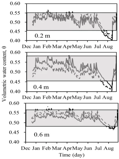
each probe. This was because the range of θ, when the soil solution was sampled, was too narrow as compared to the range of θ measured by TDR probes. As shown in Fig. 5,
θ ranged from 0.40 to 0.57 in the field, while the extracted
soil solution was in the θ range of 0.46 to 0.55 (the cor-responding TDR measurement values). The soil solution was not extracted in the period of mid-July to mid-August, when the soil was relatively dry (0.40 < θ < 0.46). When the
field data of θ exceeded the fitted range, the estimated ECw
took unrealistic values. In some cases, the estimated ECw
had negative values (from mid-July to mid-August). In the topsoil layer of 0.4 m, and the subsoil layer of 0.6 m, the discrepancy in the range of θ was not severe as compared to that at 0.2 m, and the estimation of ECw at 0.4 and 0.6 m
depth was more stable than the data obtained at a depth of 0.2 m; RMSE was 0.27, 0.22 and 0.42 dS m-1 for probes at
a depth of 0.4 m, and 0.12, 0.12 and 0.18 dS m-1 for probes
at a depth of 0.6 m. Compared with the estimation made by Miyamoto et al. (2015), which yielded RMSE of 0.42, 0.29 and 0.42 dS m-1 for probes at a depth of 0.4 m, and 0.38,
0.33 and 0.21 dS m-1 for probes at a depth of 0.6 m, the
estimation with the proposed method was more close to the
field-obtained data, especially at a depth of 0.6 m.
Figure 4 shows that the proposed method worked
fine with the subsoil layer but did not work at a depth of
0.2 m as well as expected. The main reason for failure was that we could not extract the soil solution from dry soil. Especially at the driest period of July to mid-August, the water content reached θ = 0.40 at topsoil and
θ = 0.46 at subsoil, corresponding to 100 kPa matric suction (Fig. 1). Extracting the soil solution of such high matric
suction through porous cups proved difficult.
We tried to overcome this difficulty (i.e. the unavail-ability of the dry soil solution) by adding a small amount of experimental data for our analysis. Note that in the labora-tory experiment the soil solution was centrifuged and data were available for lower water contents when compared to
the field data. As our method aims at reducing the work -load required for a laboratory experiment to be performed, we only introduced 2 data sets, i.e. (1) dry soil with small
EC and (2) wet soil with high EC. Based on the laboratory data provided by Miyamoto et al. (2015), we used these 2 data points; (1) θ = 0.35, ECa = 0.030 dS m-1, ECw = 0.49
dS m-1 (2) θ = 0.60, EC
a= 1.20 dS m-1, ECw = 3.94 dS m-1. In addition to 17 data points from the field, 2 data points
from the laboratory experiment were used for estimating the Rhoades parameter sets. For compensating the numbers
of data points in the laboratory, as compared to the field
data, weights (wi in Eq. (7)) were set as 3 for the laboratory data and 1 for the field data.
Figure 5 0.40 0.45 0.50 0.55 0.60
Dec Jan Feb Mar AprMay Jun Jul Aug
0.40 0.45 0.50 0.55 0.60
Dec Jan Feb Mar AprMay Jun Jul Aug
0.40 0.45 0.50 0.55 0.60
Dec Jan Feb Mar AprMay Jun Jul Aug Time (day)
0.2 m
0.4 m
0.6 m
Vo
lume
tric
w
ate
r c
on
ten
t,
q
Fig. 5. Volumetric water content measured at depths of 0.2, 0.4 and 0.6 m in three TDR locations (the solid line, the dashed line and the chain line representing TDR probes). The shadow area shows the range of the volumetric water content (the correspond-ing TDR value) of the extracted soil solution.
Table 2. Estimated parameters with field extracted soil solution and field measured TDR data, with supplementary laboratory data at dry and wet conditions
Depth 0.2 m
Probe ID 2A 2B 2C
a 2.0421 1.8905 2.1467
b -0.7269 -0.6339 -0.7814
ECs 0.0304 0.0000 0.0000
Figure 6 0.0 0.5 1.0 1.5 2.0 2.5
Dec Jan Feb Mar AprMay Jun Jul Aug ECw
(dS
m
-1)
Time (day)
The parameter set at the topsoil layer (0.2 m depth)
estimated in this modified method is shown in Table 2.
Figure 6 shows the change in the estimated ECw, calculated
from θ and ECa measured with TDR probes, and para-
meters in Table 2, when compared with to the ECw directly
measured from the soil solution. The estimated curve is more stable than in Fig. 4, where no laboratory data was used. RMSE was 0.37, 0.50 and 0.53 dS m-1 for each probe.
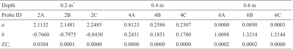
Figure 7 shows a similar result as in Fig. 4, but with
a reduced set of field data; 8 data were included out of full
dataset comprising 17 entries. As for a depth of 0.2 m, the same data from the laboratory experiment, as shown in Fig. 6, i.e., the two datasets of the dry and wet soils, were also
used in the analysis. Weights were set as 1 for both the field and laboratory data. The estimated parameter in this figure
is summarised in Table 3. By comparing the curves of Fig. 4 (for depths of 0.4 m and 0.6 m) and Fig. 6 (for a depth of 0.2 m) with Fig. 7, the estimated curves represent the
measured data equally well. In other words, decreasing the
measured data from 17 to 8 did not significantly deteriorate
the estimation, as the reduced data included the driest data in mid-July and, therefore, the range of the water content of the reduced dataset was similar to that of the whole data.
In Figs 7, 8 data out of the full set of 17 data were used. The remaining 9 data were used for the validation set. RMSE for the estimated ECw for the validation set was
0.41, 0.50 and 0.35 dS m-1 for probes at a depth of 0.2 m,
0.27, 0.25 and 0.23 dS m-1 for probes at a depth 0.4 m depth,
and 0.09, 0.12 and 0.09 dS m-1 for probes at a depth of
0.6 m. This result was not particularly higher than the RMSE of the estimation from the whole set of data; in some of the probes, RMSE got smaller. Therefore, it was
con-firmed that the estimation of Fig. 7 did not deteriorate from
Figs 4 and 6 although the numbers of data were reduced from 17 to 8.
As we have shown in the reduced set of field data,
increasing the numbers of data points (from 8 to17) does not always improve the estimation. The estimation can be improved by using as wide range of water content as pos-sible, from dry soil to wet soil, to minimise the discrepancy
of the fitted range of water content and the monitored range
of water content, as shown in Fig. 5. When it is technically
difficult to obtain a wide range of water content, laboratory
data under extreme water content conditions can be used to form an additional dataset, as shown in Fig. 6.
The estimation of ECw based on the parameter set
deter-mined under laboratory conditions (Fig. 3 in Miyamoto
et al., 2015) was improved with the proposed method, which uses the parameter set determined directly from the
field-obtained value. For example, in Miyamoto’s estima -tion, the NO3-N concentration at a depth of 0.6 m was twice
as large as the NO3-N concentration measured with the
extracted soil solution because ECw rose twice as much as
the soil solution ECw. In the proposed method, the highest
value of the estimated ECw was similar to that of the
meas-ured ECw value. Therefore, a more realistic value of NO3-N
can be obtained by the proposed method.
This is because the parameters estimated in the proposed
method (Table 1) reflect the properties found under the site-specific heterogeneous condition, and they are different
from the parameters shown in Miyamoto et al. (2015); they
are soil-specific parameters determined through a labora -tory experiment. Therefore, the parameter set obtained at
Figure 7 0.0 1.0 2.0
Dec Jan Feb Mar AprMay Jun Jul Aug
0.0 0.5 1.0 1.5 2.0 2.5
Dec Jan Feb Mar AprMay Jun Jul Aug ECw
(dS
m
-1)
0.0 0.5 1.0 1.5 2.0 2.5
Dec Jan Feb Mar AprMay Jun Jul Aug Time (day)
0.2 m
0.4 m
0.6 m
Fig. 7. Estimated ECw (the solid line, the dashed line and the chain line representing TDR probes) and the measured ECw of the extracted soil solutions (the closed and open circles represent-ing suction cups), estimated from a reduced set of field data. At a depth of 0.2 m, laboratory data under dry and wet condition was also used.
Table 3. Estimated parameters with reduced numbers of field data
Depth 0.2 m* 0.4 m 0.6 m
Probe ID 2A 2B 2C 4A 4B 4C 6A 6B 6C
a 2.1132 2.1481 2.2485 0.8123 0.2586 0.2307 0.0000 0.0890 0.0003
b -0.7660 -0.7975 -0.8430 0.2431 0.1851 0.1780 1.0088 1.3214 1.2144
ECs 0.0304 0.0001 0.0000 0.0000 0.0000 0.0000 0.0002 0.0002 0.0000
one field site by using this method should not be used for other field sites even if the soil properties are similar. The parameters determined are not soil-specific but site-specific
values.
CONCLUSIONS
1. Compared to the conventional method of estimat-ing Rhoades parameters through a laboratory experiment, the method proposed in this study, where Rhoades
param-eters are estimated based on the field-monitored values of the time domain reflectometry and the field-extracted soil
solution, can give better estimates of soil solution electri-cal conductivity. The method is reliable since it is based on the actual soil solution electrical conductivity values
measured in the field. It was made possible because our
method determines the initial parameter set for non-linear regression systematically and does not require a 2-step linear regression process as the one performed in the conventional method.
2. The key to success in this method is to obtain the soil solution of a wide range of water content. When a
suf-ficiently wide range of water content is not available in the field, a small amount of supplementary data obtained under
laboratory conditions can be added to widen the calibration range.
3. When researchers, engineers or farmers want to esti-mate the soil solution electrical conductivity accurately without much effort, the method proposed here may be
use-ful for them provided that they can access the field data of
the soil solution electrical conductivityeasily.
Conflict of interest: The authors do not declare any
conflict of interest. There is a patent pending in Japan (appli -cation number: 2018-080205) for the method described in this paper. There are no other patents.
REFERENCES
Baumgartner N., Parkin G.W., and Elrick D.E., 1994. Soil water content and potential measured by hollow time domain reflectometry probe. Soil Sci. Soc. Am. J., 58, 315-318.
Das B.S., Wraith J.M., and Inskeep W.P., 1999. Nitrate concen-trations in the root zone estimated using time domain reflectometry. Soil Sci. Soc. Am. J., 63, 1561-1570. De Neve S., van de Steene S., Hartmann R., and Hofman G.,
2000. Using time domain reflectometry for monitoring mineralization of nitrogen from soil organic matter. European J. Soil Sci., 51(2), 295-304.
Gupta S.C. and Hanks R.J., 1972. Influence of Water content on electrical conductivity of the soil. Soil Sci. Soc. Am. Proc., 36, 855-857.
Heimovaara T.J., 1995. Assessing temporal variations in soil water composition with time domain reflectometry. Soil Sci. Soc. Am. J., 59, 689-698.
Hilhorst M.A., 2000. A pore water conductivity sensor. Soil Sci. Soc. Am. J., 64, 1922-1925.
IUSS Working Group, 2014. World reference base for soil resources 2014 international soil classification system for naming soils and creating legends for soil maps. FAO, Rome.
Malicki M.A. and Walczak R.T., 1999. Evaluating soil salinity status from bulk electrical conductivity and permittivity. European J. Soil Sci., 50, 505-514.
Mallants D., Vanclooster M., Toride N., Vanderbrorght J., van Genuchten M.Th. and Feyen J., 1996. Comparison of three methods to calibrate TDR for monitoring solute movement in unsaturated soil. Soil Sci. Soc. Am. J., 60, 747-754.
Marquardt D.W., 1963. An algorithm for least-square estimation of nonlinear parameters. J. Soc. Industrial Appl. Mathe- matics, 11(2), 431-441.
Miyamoto T., Kameyama K., and Iwata Y., 2015. Monitoring electrical conductivity and nitrate concentrations in an Andisol field using time domain reflectometry. Japan Agric. Res. Quarterly, 49(3), 261-267.
Mualem Y. and Friedman S.P., 1991. Theoretical prediction of electrical conductivity in saturated and unsaturated soil. Water Res. Res., 27, 2771-2777.
Muñoz-Carpena R., Regalado, C.M., Ritter A., Alvarez-Benedi J., and Socorro A.R., 2005. TDR estimation of electrical conductivity and saline solute concentration in a volcanic soil. Geoderma, 124, 399-413.
Noborio K., 2001. Measurement of soil water content and electri-cal conductivity by time domain reflectometry: a review. Computers and Electronics in Agriculture, 36, 113-132. Risler P.D., Wraith J.M., and Gaber H.M., 1996. Solute
trans-port under transient flow conditions estimated using time domain refrectometry. Soil Sci. Soc. Am. J., 60, 1297-1305.
Rhoades J.D., Manteghi N.A., Shouse P.J., and Alves W.J., 1989. Soil electrical conductivity and soil salinity: New for-mulations and calibrations. Soil Sci. Soc. Am. J., 53, 433-439.
Rhoades J.D., Raats P.A., and Prather R.J., 1976. Effects of liquid-phase electrical conductivity, water content, and sur-face conductivity on bulk soil electrical conductivity. Soil Sci. Soc. Am. J., 40, 651-655.
Scudiero E., Berti A., Teatini P., and Morari F., 2012. Simultaneous monitoring of soil water content and salinity with a low-cost capacitance-resistance probe. Sensors, 12, 17588-17607.
Seki K., 2007. SWRC fit – a nonlinear fitting program with a wa-ter retention curve for soils having unimodal and bimodal pore structure. Hydrology Earth System Sci. Discussions, 4(1), 403-437.
Šimůnek J. and Hopmans J.W., 2002. Parameter Optimization and Nonlinear Fitting. in Methods of Soil Analysis: Part 4 Physical Methods, 139-158. Soil Science Society of America, Madison, WIS, USA.
Vaz C.M.P., Jones S., Meding M., and Tuller M., 2013. Evaluation of standerd calibration function for eight elec-tromagnetic soil moisture sensors. Vadose Zone J., 12(2), doi: 10.2136/vzj2012.0160.