Existence and Uniqueness Solutions of Fuzzy Integration-Differential Mathematical Problem by Using the Concept of Generalized Differentiability

Vol. 17, No. 1, 2019, 21-40

ISSN: 2320 –3242 (P), 2320 –3250 (online) Published on 10 April 2019

www.researchmathsci.org

DOI: http://dx.doi.org/10.22457/196ijfma.v17n1a3

21

International Journal of

Existence and Uniqueness Solutions of Fuzzy

Integration-Differential Mathematical Problem by Using the Concept

of Generalized Differentiability

1,3

Department of Mathematics, Science and Research Branch Islamic Azad University, Tehran, Iran

2

Department of Mathematics, Ardabil Branch Islamic Azad University, Ardabil, Iran 2

Corresponding author, Email: [email protected]

Received 28 February 2019; accepted 25 March 2019

Abstract. In this study, we demonstrate studies on two type of solutions linear fuzzy functional integration and differential equation under two kinds Hukuhara derivative byusing the concept of generalized differentiability. Various types of solutions to are generated by applying of two separate concepts of Fuzzy derivative in formulation of differential problem. Some patterns are presented to describe these results.

Keywords: Existence and uniqueness solutions, integration-differential mathematical problem, generalized differentiability

AMS Mathematics Subject Classification (2010):34A07

1. Introduction

The theory of calculus, which deals with the investigation and applications of derivatives and integrals of arbitrary order has a long history. The theory of calculus developed mainly as a pure theoretical field of mathematics, in the last decades it has been used in various fields as rheology, viscoelasticity, electrochemistry, diffusion processes, etc [32, 33].calculus have undergone expanded study in recent years as a considerable interest both in mathematics and in applications. One of the recently influential works on the subject of calculus is the monograph of Podlubny [49] and the other is the monograph of Kilbas et al. [33]. The differential equations have great application potential in modeling a variety of real world physical problems, which deserves further investigations. Among these we might include the modeling of earthquakes, the fluid dynamic traffic model with derivatives, the measurement of viscoelastic material properties, etc. Consequently, several research papers were done to investigate the theory and solutions of differential equations (see [18, 21, 35, 37] and references therein).

The concept of solution for differential equations with uncertainty was

Riemann-22

Liouville differentiability. Some existence results for nonlinear fuzzy differential equations of order involving the Riemann-Liouville derivative have been proposed in [30]. The solutions of fuzzy differential equations are investigated by using the fuzzy Laplace transforms in [51]. Recently, the concepts of derivatives for a fuzzy function are either based on the notion of Hukuhara derivative [25] or on the notion of strongly generalized derivative. The concept of Hukuhara derivative is old and well known, but the concept of strongly generalized derivative was recently introduced by Bede and Gal [13]. Using this new concept of derivative, the classes of fuzzy differential equations have been extend and studied in some papers such as: Ahmad et al. [4], Allahviranloo et al. [9]-[11], Bede et al. [14]-[17], Gasilov [20], Khastan et al. [27]-[29], Malinowski [41]-[43] and Nieto [46]. Furthermore, by using this new concept of derivative, Allahviranloo et al. in [7, 8] have studied the concepts about generalized Hukuhara Riemann-Liouville and Caputo differentiability of fuzzy valued functions. Later, authors have proved the existence and uniqueness of solution for fuzzy differential equation by using different methods. Alikhani et al. in [6] have proved the existence and uniqueness results for nonlinear fuzzy integral and integration and differential equations by using the method of upper and lower solutions. Mazandarani et al. [44] studied the solution to fuzzy initial value problem under Caputo-type fuzzy derivatives by a modified Euler method. Besides, authors studied some results on the existence and uniqueness of solution to fuzzy differential equation under Caputo type-2 fuzzy derivative and the definition of Laplace transform of type-2 fuzzy number-valued functions [45]. Salahshour et al. [50] proposed some new results toward existence and uniqueness of solution of fuzzy differential equation. According to the concept of Caputo-type fuzzy derivative in the sense of the generalized fuzzy differentiability, Fard et al. [19] extended and established some definitions on fuzzy calculus of variation and provide some necessary conditions to obtain the fuzzy Euler-Lagrange equation for both constrained and unconstrained fuzzy variational problems. Ahmad et al. [5] proposed anew interpretation of fuzzy differential equations and present their solutions analytically and numerically. The proposed idea is a generalization of the interpretation given in [3, 4], where the authors used Zadeh’s extension principle to interpret fuzzy differential equations.

In real world systems, delays can be recognized everywhere and there has been

widespread interest in the study of delay differential equations for many years. Therefore, delay differential equations (or, as they are called, functional differential equations) play an important role in an increasing number of system models in biology, engineering, physics and other sciences. There exists an extensive amount of literature dealing with delay differential equations and their applications; the reader is referred to the monographs [22, 34], and the references therein. The study of fuzzy delay differential equations is expanding as a new branch of fuzzy mathematics. Both theory and applications have been actively discussed over the last few years. In the literature, the study of fuzzy delay differential equations has several interpretations. The first one is based on the notion of Hukuhara derivative. Under this interpretation, Lupulescu established the local and global existence and uniqueness results for fuzzy delay differential equations. The second interpretation was suggested by Khastan et al. [29] and Hoa et al. [24].

In this setting, Khastanetal proved the existence of two fuzzy solutions for fuzzy

23

established the global existence and uniqueness results for fuzzy delay differential equations using the concept of generalized differentiability. Moreover, authors have extended and generalized some comparison theorems and stability theorem for fuzzy delays differential equations with definition a new Lyapunov-like function. Besides that, some very important extensions of the fuzzy delay differential equations In [21, 28, 35, 53], the authors considered the fuzzy differential equation with initial value

_{= . .}

= . 1.1

where f : [0, ∞) × Ed→ Ed and the symbol ′denotes the first type Hukuhara derivative (classic Hukuhara derivative). O. Kaleva also discussed the properties of differentiable fuzzy mappings in [28] and showed that if f is continuous and f (t, x) satisfies the Lipschitz condition with respect to x, then there exists a unique local solution for the fuzzy initial value problem (1.1). Lupulescu proved several theorems stating the existence, uniqueness and boundedness of solutions to fuzzy differential equations with the concept of inner product on the fuzzy space under classic Hukuhara derivative in [35].

In [34], Lupulescu considered the fuzzy functional differential equation _{= −} = . . ≥

∈ . ≥ ≥ − (1.2) where f : [0, ∞) × Cσ→ Ed and the symbol ′denotes the first type Hukuhara derivative (classic Hukuhara derivative). Author studied the local and global existence and uniqueness results for (1.2) by using the method of successive approximations and contraction principle.

In this paper, we consider fuzzy functional integration and differential equations under form

D = . + . !. "_& #$%. ≥

= − = ∈ '( . ≥ ≥ −

(1.3)

We establish the local and global existence and uniqueness results for (1.3) by using the method of successive approximations and contraction principle. This direction of research is motivated by the results of Bede and Gal [17], Chalco-Cano and Roman-Flores [23], Malinowski [37-40], Ahmad, Sivasundaram [1], Allahviranloo et al. [5-7]. The paper is organized as follows. In Section 2, we collect the fundamental notions and facts about fuzzy set space, fuzzy differentiation and integration. In Section 3, we discuss the FFIDEs with a two kinds of fuzzy derivative. Some examples of this class having two different solutions were presented in Section 4.

2. Preliminaries and notation

In this section, we give some notations and properties related to fuzzy set space, and summarize the major results for integration and differentiation of fuzzy set-valued mappings. We recall some notations and concepts presented in detail in recent series works of Lakshmikantham et al. [32, 33].

Let Kc(R d

) denote the collection of all nonempty compact and convex subsets of Rd and scalar multiplication in Kc(R

d

) as usual, i.e. for A, B ∈Kc(R d

) and λ ∈ R. A + B = {a + b | a ∈A, b ∈B}, λA= {λa| a ∈A}.

The Hausdorff distance $in Kc(Rd) is defined as follows

24

where A, B ∈(Kc,Rd), ‖. ‖_:;denotes the Euclidean norm in Rd. It is known that (Kc,Rd), $

is a complete metric space. Denote Ed= {ω : Rd→ [0, 1] such that ω(z) satisfies (i)-(iv) stated below}

i. ω is normal, that is, there exists z0∈ Rdsuch that ω(z0) = 1;

ii. ω is fuzzy convex, that is, for 0 ≤ λ ≤ 1 ω(λz1 + (1 - λ)z2) ≥ min{ω(z1), ω(z2)}, for any z1, z2 ∈ Rd;

iii. ω is upper semi continuous;

iv. [ω]0= cl{z ∈ Rd: ω(z) >0} is compact, where cl denotes the closure in (Rd, ‖. ‖). Although elements of Edare often called the fuzzy numbers, we shall just call them the fuzzy sets.

For α ∈(0, 1], denote [ω]α= {z ∈Rd| ω(z) ≥ α}. Wewill call this set an α-cut ( α- level set) of the fuzzy set ω. For ω ∈Ed one has that [ω]α∈Kc(Rd)for every α ∈[0, 1]. For two fuzzy ω1, ω2 ∈Ed, we denote ω1 ≤ ω2 if and only if [ω1]α⊂[ω2]α.

If g : Rd× Rd→ Rd is a function then, according to Zadeh’s extension principle, one can extend

g to Ed × Ed → Ed by the formula g(ω1, ω2)(z) =supz=g(z1,z2)min {ω1(z1), ω2(z2)} . It is well known that if g is continuous then [g(ω1, ω2)]α= g([ω1]α, [ω2]α)for all ω1, ω2 ∈Ed, α ∈ [0, 1]. Especially, for addition and scalar multiplication in fuzzy set space Ed, we have [ω1 + ω2]α= [ω1]α+ [ω2]α, [λω1]α=λ[ω1]α. The notation [ω]α= [ω(α), ω(α)]. We refer to ω and ω as the lower and upper branches of ω, respectively.

For ω ∈Ed, we define the length of ω as len(ω) =ω(α) - ω(α)In the case d = 1, we have len(ω) = ω(α) - ω(α). Let us denote =[ω1, ω2] = sup{dH([ω1]α, [ω2]α) : 0 ≤ α ≤ 1} the distance between ω1 and ω2 in Ed, where dH([ω1]

α

, [ω2]α) is Hausdorff distance between two set[ω1]α, [ω2]α of (Kc,Rd). Then (Ed, dH) is a complete space. Some properties of metric D are as follows.

=[ω1 + ω3, ω2 + ω3] = =[ω1, ω2],=[λω1, λω2] = |λ|=[ω1, ω2],=[ω1, ω2] ≤

=[ω1, ω3] + =[ω3, ω2], for all ω1, ω2, ω3 ∈Ed and λ ∈R. Let ω1, ω2 ∈Ed. If there exists ω3 ∈Ed such that ω1 = ω2 + ω3 then ω3 is called the difference of ω1, ω2 and it is denoted ω1Өω2. Let us remark that ω1 Өω2 ≠ ω1 + (-1)ω2.

Remark 2.1. If for fuzzy numbers ω1, ω2, ω3 ∈Ed there exist Hukuhara difference ω1Өω2, ω1 Өω3 then=[ω1Өω2, 0] = =[ω1, ω2] and =[ω1 ω2, ω1Өω3] = =[ω2, ω3].

The strongly generalized differentiability was introduced in [17] and studied in [18, 23, 42].

Definition 2.1. (See [17]) Let x: (a, b) → Ed and t ∈(a, b). We say that x is strongly generalized differentiable at t, if there exists DHgx(t)∈Ed, such that either (i) for all h >0 sufficiently small, the differences x (t + h) Өx(t), x(t) Өx(t - h) exist and the limits (in the metric =)

?3@

ℎ ↘ 0D + ℎ ⊖ _ℎ = ?3@_{ℎ ↘ 0}D + ℎ ⊖ _ℎ = D or

25 ?3@

ℎ ↘ 0D ⊖ + ℎ_−ℎ = ?3@_{ℎ ↘ 0}D − ℎ ⊖ _−ℎ = D or

(iii) for all h >0 sufficiently small, the difference x (t + h) Өx(t),∃x(t - h) Өx(t) exist and the limits

?3@

ℎ ↘ 0D + ℎ ⊖ _ℎ = ?3@_{ℎ ↘ 0}D − ℎ ⊖ _−ℎ = D

(iv) for all h >0 sufficiently small, the difference x (t) Өx(t + h), ∃x(t) Өx(t - h) exist and the limits

?3@

ℎ ↘ 0D ⊖ + ℎ_−ℎ = ?3@_{ℎ ↘ 0}D ⊖ − ℎ_ℎ = D .

In this definition, case (i) ((i)-differentiability for short) corresponds to the classic derivative, so this differentiability concept is a generalization of the Hukuhara derivative. In Ref. [17], Bede and Gal consider four cases for derivative. In this paper we consider only the two first of Definition 2.1. In the other cases, the derivative is trivial because it is reduced to a crisp element.

Lemma 2.1. (Bede and Gal [17]) If x(t) =(z1(t), z2(t), z3(t)) is triangular number valued function, then

(i) if x is (i)-differentiable (i.e. Hukuhara differentiable) then DH g x(t) = (z´ 1(t), z´2(t), z´3(t));

(ii) if x is (ii)-differentiable then DH g x(t) = (z´ 3(t),z´ 2(t), z´1(t)).

Lemma 2.2. (see [23]) Let x ∈E1and put [x(t)]α =[x(t, α), x(t, α)] for each α∈ [0, 1]. (i) If x is (i)-differentiable then x(t, α), x(t, α) are differentiable functions and we have

[D ]I_{= J. K. . KL ∙ (2.4)}

(ii) If x is (ii)-differentiable then x(t, α), x(t, α) are differentiable functions and we have:

(iii) [D ]I= J. K. . KL (2.5)

Definition 2.2. [52] A point t ∈ (a, b), is a switching for the differentiability of x, if in any neighborhood V of t there exist points t1 < t < t2 such that

(type I) at t1 (2.4) holds while (2.5) does not hold and at t2 (2.5) holds and (2.4) not hold, or

(type II) at t1 (2.5) holds while (2.4) does not hold and at t2 (2.4) holds and (2.5) not hold.

Lemma 2.3. Let a(t),b(t) and c(t) be real valued nonnegative continuous functions defined on R+, d ≥ 0 is a constant for which the inequality

a t ≤ $ + P Q5 !2 ! + 5! P RS2 S$S

T $%

26 a t ≤ $ + Q1 + P 5 %U1

VP 5S + R S$S

W

X $% ∙T

3. Main results

For σ >0 let Cσ= C([-σ, 0], Ed) denote the space of continuous mappings from [-σ, 0] to Ed. Define a metric Dσ in Cσ by

=([. Y] = _{∈ [−Z. 0=}%01 [. Y] ∙

Let p >0. Denote I = [t0, t0+ p], J =[t0- σ, t0] ∪I = [t0- σ, t0+ p]. For any t ∈I denote by the

element of Cσ defined by xt(s)= x(t + s) for s ∈[-σ, 0].

Let us consider the fuzzy functional integration and differential equations (FFIDEs) with generalized Hukuhara derivative under form

D = . + . %. _& W$%. ≥

= − = ∈ '(. ≥ ≥ −

(3.1)

where f :I × Cσ→ Ed, g : I × I × Cσ→ Ed, ϕ ∈Cσ and the symbol DHg denotes the generalized Hukuhara derivative from Definition (2.1). By a solution to equation (3.1) we mean a fuzzy mapping x ∈C(J, Ed), that satisfies:

X(t) = (t - t0) for t ∈[t0-σ, t0], x is differentiable on [t0, t0+ p] and

= = . + . %. _W$%. \S ∈ ] &

Lemma 3.1. Assume that f ∈C(I × Cσ, Ed), g ∈C(I × I × Cσ, Ed) and x ∈C(J, Ed). Then the fuzzy mapping

→ . + P . %. W$%

& Belongs to C(I, Ed).

Remark 3.1. Under assumptions of the lemma above we have the mapping

→ . + P . %. W$%

& Is integrable over the interval I.

Remark 3.2. If f: I × Cσ→ Ed, g : I × I × Cσ→Ed are jointly continuous functions and x ∈C(J, Ed), then the mapping

→ . + P . %. W$%

&

Is bounded on each compact interval I. Also, the function

→ . + P . %. W$%

& is bounded on I.

27

_ _{= 0 `%.} = . \S ∈ [− . ]

W + . %. _& W$%a

& $% ∈ ].

(3.4) if x is (i)-differentiable or (iii)-differentiable.

b

= − \S ∈ [− . ]

= 0 ⊖ −1

× `%. _& W + . %. _& W$%a$% ∈ ].

(3.5)

if x is (ii)-differentiable or (iv)-differentiable. Let us remark that in (3.5) it is hidden the following statement: there exists Hukuhara difference ϕ(0)Ɵ

−1 P V%. W + P . %. W$%

&

X

&

$%

Definition 3.1. Let x :J → Ed be a fuzzy function such that (i)-differentiable. If x and its derivative satisfy problem (3.1), we say that x is a (i)-solution of problem(3.1).

Definition 3.2. Let x :J → Ed be a fuzzy function such that (ii)-differentiable. If x and its derivative satisfy problem (3.1), we say that x is a (ii)-solution of problem (3.1).

Definition 3.3. A solution x :J → Ed is unique if it holds D0[x(t), y(t)] = 0, for any y : J →

Ed which is a solution of (3.1).

Theorem 3.1. Let (t - t0) ∈Cσ and suppose that f ∈C(I × Cσ, Ed),g ∈C(I × I × Cσ, Ed)

satisfy the condition: there exists a constant L >0 such that for every ξ, ψ ∈Cσ it holds maxd=[. e. . f]. =[ . %. e. . %. f]g ≤ h [e. f]

Moreover, there exists a M >0 such that max{D0[f(t,ξ),0], D0[g(t,s,ξ),0}<=M

Assume that the sequence {xn}∞n=0, xn: J → Ed given by _{= −} . ∈ [− . ]

0. ∈ ].

and for n = 1, 2, ...

8Di ₌

__{0 ⊖ −1 `%.} − . ∈ [− . ]

W8 + %. Z. _& j8$Za

& $% ∈ ].

(3.4) is well defined, i.e. the foregoing Hukuhara difference do exist. Then the FFIDE (3.1) has a unique for each case ((i)-differentiable or (ii)-differentiable).

Proof: From assumptions of this Theorem we have D0[x1(t), x0(t)]= =[i. ]

= = [0 ⊖ −1 × `%. <sub>&</sub> W + %. Z. W<sub>&</sub> j$Za$%. 0] ≤ `=_& J%. W. 0kL + =W_& J %. Z. j. 0kL$Za$%

≤ l − + l − m

2! .

28

= = [⊖ −1 P V%. W8 + P %. Z. j$Z W & X & $%.

⊖ −1 `%. _& W8pi + %. Z. W_& j8pi$Za$%] ≤ h P V=([W8. W8pi] + P =([j8. j8pi]$Z

W & X & $%.

≤ h P ` _{q ∈ [−. 0]}%01

&

= [8% + q. 8pi% + q]

+ PW_{q ∈ [−. 0]}%01

&

= [8Z + q. 8piZ + q]$Z$%

= h P ` _{S ∈ [% − . %]}%01

&

= [8S. 8piS]

+ PW_{r ∈ [Z − . Z]}%01

&

= [8r. 8pir]$r$S

In particular, from (3.4), we get

=[m. i] ≤ hl V − m

2! + 2 − s

3! + − u

4! X Therefore, by mathematical induction, for every n ∈N and t ∈I

=[8Di. 8]

≤ hl8_V − 8Di

4 + 1! +8wi − 8Dm

4 + 2! + ⋯ +8w8 − m8Di

24 + 1! + −

m8Dm

24 + 2! X In the inequality (3.5), λ1, . . . ,λn are balancing constants. We observe that for every n∈ {0, 1, 2, . . .}, the function xn(·) : J → Ed are continuous. Indeed, since∈Cσ, x0(t) is continuous on t∈[-σ, t0+ p]. We see that

=[i + ℎ. i] = =

y z z z z z

{ 0 ⊖ −1

× P

V%. W + P %. Z. j$Z W

&

X $%. 0 ⊖ −1

× P %.

&

W + P %. Z. j$Z W & $% D| & } ~ ~ ~ ~ ~ 

Thus, by mathematical induction, for every n ≥ 2, we deduce that D0[x

n

(t + h), xn(t)] → 0 as h → 0+. A similar inequality is obtained for D0[x

n

(t - h), xn(t)]

→ 0 as h → 0+. In the sequel we shall show that for the {xn(t)} the Cauchy convergence condition is satisfied uniformly in t, and as a consequence{xn(·)} is uniformly convergent. For n > m >0, from (3.5) we obtain

%01

∈ ]=[8. €] = %01 _{∈ =}[8. €]

≤ ‚ _{∈ }%01

8pi

ƒ„€

29 ≤ l ‚ V − _{† + 1! +}ƒDi 8_wi − ƒDm

† + 2! + ⋯ +ƒwƒ − mƒDi

2† + 1! + −

mƒDm

2† + 2! X

8pi

ƒ„€

The convergence of this series implies that for any ε >0we find n0∈N large enough such

that for n, m > n0

=[8. €] < ˆ 3.6 Since (Ed, =) is a complete metric space and (3.6)holds, the sequence {xn(·)} is uniformly convergent to a mapping x ∈C(J, Ed). We shall that x is a solution to (3.1). Since xn(t) = (t - t0) for every n = 0, 1, 2, ...and every t ∈[t0- σ, t0], we easily have x(t) =

(t -t0). For s ∈I and n ∈N

=QP %.

&

W8$%. P %. W$%

&

T

≤ h P_{q ∈ [% − . %]}%01

&

=[8q. q]$q → 0

And

= [P P %. Z. j8. $Z$% W

&

&

. P P %. Z. j. $Z$% W

&

&

]

≤ h PP_{q ∈ [Z − . Z]}%01

&

&

=[8Š. Š]$Š$% → 0

As n→∞ for any t ∈I. Consequently, we have

=[0. + −1 P%. W +

&

P . %. W$%$%

&

]

≤ =[8. ]

+ P= [%. W8pi + %. W]

&

+ P= [ %. Z. j8pi. %. Z. j$Z]

&

$%

We infer that

=‹0. + −1 P%. W +

&

P . %. W$%$%

&

Π= 0

for every t ∈I. Therefore x is the solution of (3.3), due to Lemma (3.2) we have that x is a (ii)-solution of (3.1). For the uniqueness of the solution x let us assume that x, y ∈C(J, Ed) are two solution of (3.3). By definition of the solution we have x(t) = y(t) if t ∈[t0- σ, t0].

Note that for t∈I

30

≤ h P_{q ∈ [% − . %]=}%01 [q. Yq]

&

+ P `_{r ∈ [Z − . Z]=}%01 [r. Yr]$Za$%

&

If we let a(s) = sup r∈[s-σ,s]D0 [x(r), y(r)] , s ∈ [t0, t] ⊂[t0, t0+ p], then we have

2 ≤ h P 2% + P 2Z$Z

W

&

Ž $%

&

and by Lemma 2.3 we obtain that a(t) = 0 on I. This prove the uniqueness of the solution for (3.1).

Remark 3.3. The existence and uniqueness theorem for the problem (3.1) can be obtained using the contraction principle.

Now, we shall prove existence and uniqueness results for (3.1) by using the contraction principle, which studied in [34]. In the following, for a given k >0, we consider the set Sk of all continuous fuzzy functions

x ∈C([t0- σ, ∞), Ed) such that x(t) = (t - t0) =x0 on [t0- σ, t0] and

supt≥t0-σ{D0[x(t, ω), 0] exp( ˆ -kt) <∞.

On Sk we can define the following metric

=ƒ[. Y] = _≥ %01_{− d=}[. Y] exp−†g 3.7

Where k>0 is chosen suitably later. We easily prove that the space [Sk, Dk] of continuous fuzzy functions x: [t0, ∞) → Ed is a complete metric space with distance (3.7).

Theorem 3.2. Assume that (i) f ∈C([t0, ∞) × Cσ, E

d

), g ∈C([t0, ∞) ×[t0, ∞) × Cσ, E

d

) and there exists a constant L >0 such that

(ii) @2 d=[. e. . f]. d=[ . %. e. . %. f] ≤ h=₍[e. f] for all ξ, ψ ∈Cσ and t, s ≥ t0;

(iii) there exists constants M >0 and b >0 such that

@2 d=[. 0k. 0k]. = . %. 0k. 0k]g ≤ l exp 5

for all t ≥ t0, where b < k. Then the FFIDE (3.1) has a unique solution for each case on

[t0, ∞).

Proof: Since the way of the proof is similar for all four cases, we only consider case (ii)-differential for x. In this case, we consider the complete metric space (Sk, Dk), and define an operator T :Sk→ Sk x → Tx

given by

’ =

“ ” • ”

– d − _{0 ⊖ −1} 3 ∈ [− . ]

× P%. W +

&

P %. Z. W$Z$%

&

31

We can choose a big enough value for k such that T is a contraction, so the Banach fixed point theorem provides the existence of a unique fixed point for T, that is, a unique solution for (3.1).

Step 1: We shall prove that T(Sk)⊂Sk with assumption k > b. Indeed, let x ∈Sk. For each t

≥ t0, we get

=ƒ [ ’. 0k]

= _≥ %01 d=[0 ⊖ −1 P%. W

&

+ P %. Z. j$Z$%. W

&

0k] U%1 −†g

≤ _≥ %01 d=[0. 0k + Pd=[%. W. %. 0k]

&

+=[%. 0k. 0k]g$%

+ PPd=[ %. Z. j. %. Z. 0k] W

&

&

+ =[ %. Z. 0k. 0k]g $Z$%exp −†g

≤ _≥ %01 d=[0. 0k + h Pd=(JW. 0kL$%

&

+l_{5 exp5 + h P P =}(Jj. 0kL$Z W

&

Ž $%

&

+₅l_mexp5 exp−†g

Since x ∈Sk, there exists ρ such that supt≥t0-σ{D0[x(t), 0] exp(-kt)} < ρ <∞. Therefore, for

all t ≥ t0, we obtain =ƒ [ ’. 0]

≤ _≥ %01 d=[0. 0k + —1 +1_†˜1h_{† exp†}

+ —1 +1_5˜l_{5 exp5 exp−†g} ≤ =[0. 0k] + —1 +1_5˜1_{5 l + 1h}

≤ ™ + —1 +1_5˜1_{5 l + 1h < ∞} We infer that Tx⊂Sk.

• Step 2: The following steps, we shall prove that T is a contraction by metric Dk. The first, we consider Let x, y ∈Sk. Then for -σ ≤ s ≤ 0, D0[(Tx)(t0+s), (Ty)(t0+ s)] = 0. For

each t ≥ t0, we have=ƒ [’. ’Y]

≤ _≥ %01 d=[’. ’Y] exp−†

≤ %01

d=[0 ⊖ −1 P%. W

&

+ P %. Z. j$Z$%. W

32 0 ⊖ −1 P%. YW +

&

P %. Z. Yj$Z$%] W

&

× exp−†g

≤ _≥ %01 dh P=([W. YW] +

&

P =([j. Yj]$Z$% W

&

× exp−†g

= %01 dh P_{q[−. 0]=}%01 [% + q. Y% + q]$%

&

+h P P_{q[−. 0]=}%01 [Z + q. YZ + q W

&

]$%

&

× exp−†g

= %01 dh P_{S[% − . %]=}%01 [S. YS]$S

&

+h P P_{Š[Z − . Z]=}%01 [Š. YŠ W

&

]$Š$%

&

× exp−†g

≤ h=ƒ[. Y] _≥ %01 PU1 †S −

&

+ P exp† Š −

W

&

$Š$S

≤ 1 + †h=_†mƒ [. Y]

Choosing k > b and (1 + k) L/k2 <1, we have the operator T on Sk is a contraction by using Banach fixed point theorem provides the existence of a unique fixed point for T and the unique fixed of T is in the space Sk, that is a unique solution for (3.1) in case (ii)-differentiable and for each case.

4. Illustrations

In this section, we shall present some examples being simple illustrations of the theory of FFIDE. We will consider the FFIDE (3.1) with (i) and (ii) derivative, respectively. Let us start the illustrations with considering the following fuzzy functional integration and differential equation:

D = . + †. %_& W$%. ≥

= − ∈ . ∈ [−. ].

(4.1)

33 “

” • ”

–. K = `. K. K. Ka + †. %_& WK $%.

≥

. K = − . K. − ≤ ≤

. K = − . K. − ≤ ≤

(4.2)

If x(t) is (ii)-differentiable, then [DHg x(t)]α=[x´(t, α), x´(t, α)] and (4.1) is translated into the following delay integration and differential system:

“ ” ” • ” ”

–. K = `. K. K. Ka + †. %_& WK $%.

≥

_{. K = `. K. K. Ka + †. % WK}

& $%.

≥

. K = − . K. − ≤ ≤

. K = − . K. − ≤ ≤

(4.3)

†. %WK = †. %WK . †. % ≥ 0 .

†. %WK. †. %. < 0

†. %WK = †. %_{†. %}WK . †. % ≥ 0 . WK. †. %. < 0

Example 4.1. Let us consider the linear fuzzy functional integration and differential equation under two kinds Hukuhara derivative

“ ” • ”

–D _{= −} 1

2 + w P UWp

—% − 1_{2˜ $%}

= . ∈ ›−1_{2 .0œ .} 4.4

where k(t, s) = λe(s-t), (t) = (1 - t, 2 - t, 3 -t), λ ∈R\{0}. In this example we shall solve (4.4) on [0, 1/2].

Case 1: (λ >0 or k(t, s) >0) From (4.2), we get

“ ” ” ” ” ” • ” ” ” ” ”

–_{. K = —. −}1

2 . K˜ + w P UWp

—% − 1_{2 . K˜ $%.} ≥ 0

. K = —. −1_{2 . K˜ + w P U}Wp

—% − 1_{2 . K˜ $%.} ≥ 0

. K = 1 + K − . −1_{2 ≤ ≤ 0}

. K = 3 − K − .−1_{2 ≤ ≤ 0}

34

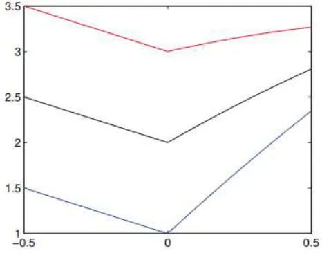
where α∈[0, 1]. By solving delay integration and differential systems (4.5), we obtain (i)-solution

[]I_{= [1 + K + 1 + K −} m

2 − w Up 2 + K +w2 + K − . 3 − K + 3 − K − ₂m

−w Up_{4 − K + w 4 − K − ].}

Figure 1: Graphs of x(t) for t ∈[1-2و1/2-], λ = 0.1.

t∈ [0, 1/2]. The (i)-solution of (4.4) on [-1/2, 1/2] are illustrated in Fig. 1.From (4.3), we obtain

“ ” ” ” ” • ” ” ” ”

–_{. K = —. −}1

2 . K˜ + w P UWp

—% − 1_{2 . K˜ $%.} ≥ 0

. K = 1 + K − .−1_{2 ≤ ≤ 0} ≥ 0

. K = 1 + K − .−1_{2 ≤ ≤ 0}

. K = 3 − K − .−1_{2 ≤ ≤ 0}

4.6

By solving delay integration and differential systems (4.6), we obtain (ii)-solution

[]I_{= [1 + K + 3 − K −} m

2 − w Up 4 − K +w4 − K − . 3 − K + 1 + K − ₂m

−w Up_{2 + K + w 2 + K − ].}

35

Figure 2: Graphs of x(t) for t ∈[1-2و1/2-], λ = 0.1.

Case 2: (λ<0 or k(t, s) <0) From (4.2), we get

“ ” ” ” ” ” • ” ” ” ” ”

–_{. K = —. −}1

2 . K˜ + w P UWp

—% − 1_{2 . K˜ $%.} ≥ 0

. K = −1_{2 . K + w P U}Wp

—% − 1_{2 . K˜ $%.} ≥ 0

. K = 1 + K − .−1_{2 ≤ ≤ 0}

. K = 3 − K − .−1_{2 ≤ ≤ 0}

4.7

By solving delay integration and differential systems (4.7), we obtain (i)-solution

[]I_{= [1 + K + 1 + K −} m

2 − w Up 4 − K

36

Figure 3: Graphs of x(t) for t ∈ [1/2و1/2-], λ = 0.1.

From (4.3), we obtain

“ ” ” ” ” ” • ” ” ” ” ”

–_{. K = —. −}1

2 . K˜ + w P UWp

—% − 1_{2 . K˜ $%.} ≥ 0

_{. K = −}1

2 . K + w P UWp

—% − 1_{2 . K˜ $%.} ≥ 0

. K = 1 + K − .−1_{2 ≤ ≤ 0}

. K = 3 − K − .−1_{2 ≤ ≤ 0}

4.8

By solving delay integration and differential systems (4.7), we obtain (ii)-solution

[]I_{= [1 + K + 3 − K −} m

2 − w Up 2 + K

37

Figure 4: Graphs of x(t) for t ∈[1/2و1/2-], λ = 0.1.

The Figs. 1 and 3. However, if we consider the second type Hukuhara derivative ((ii)- differentiable) the length of solutions change. Under the second type Hukuhara differentiable solutions have non-increasing length of its values (see Figs. 2 and 4).

5. Conclusions

In this paper, we have obtained a global existence and uniqueness result for a solution to fuzzy functional integration and differential equations. Also, we have proved a local existence and uniqueness results using the method of successive approximation. Results here might be used in further research on fuzzy functional integration and differential equations. Other possible directions of research could be an approach for fuzzy differential equations using other concepts of calculus for fuzzy functions and derivative for fuzzy functions (see [3, 8]).

Acknowledgment. The authors would like to express his gratitude to the anonymous referees for their helpful comments and suggestions, which have greatly improved the paper. This research is funded by Vietnam National Foundation for Science and Technology Development (NAFOSTED).

REFERENCES

1. B.Ahmad and S.Sivasundaram, Dynamics and stability of impulsive hybrid set valued integration and differential equations with delay, Nonlinear Analysis: Theory, Methods & Applications, 65 (2006) 2082–2093.

2. A.Ahmadian, M.Suleiman, S.Salahshour and D.Baleanu, A Jacobi operational matrix for solving a fuzzy linear differential equation, Advances in Difference Equations, 2013 (2013) 104.

38

4. R.P.Agarwal, D.O’Regan and V.Lakshmikantham, Viability theory and fuzzy differential equations, Fuzzy and Systems, 151 (2005) 536–580.

5. T.Allahviranloo, S.Abbasbandy, O.Sedaghatfar and P.Darabi, A new method for solving fuzzy integration and differential equation under generalized differentiability, Neural Computing and Applications, 21 (2012) 191–196.

6. T.Allahviranloo, S.Hajighasemi, M.Khezerloo, M.Khorasany and S.Salahshour, Existence and uniqueness of solutions of fuzzy Volterra integration and differential equations, IPMU 2010, Part II, CCIS 81 (2010) 491–500.

7. T.Allahviranloo, A.Amirteimoori, M.Khezerloo and S.Khezerloo, A new method for solving fuzzy volterra integration and differential equations, Australian Journal of Basic and Applied Sciences, 5 (2011) 154–164.

8. T.Allahviranloo, S.Salahshour and S.Abbasbandy, Solving fuzzy differential equations by fuzzy Laplace transforms, Communications in Nonlinear Science and Numerical Simulation, 17 (2012) 1372–1381.

9. T.Allahviranloo, S.Abbasbandy, O.Sedaghatfar and P.Darabi, A new method for solving fuzzy integration and differential equation under generalized differentiability, J Neural Computing and Applications, 21 (2012) 191–196.

10. T.Allahviranloo, M.Ghanbari and E.Haghi, A.Hosseinzadeh and R.Nouraei, ”A note on ”Fuzzy linear systems”, Fuzzy Sets and Systems, 177 (2011) 87–92.

11. T.Allahviranloo, S.Abbasbandy, N.Ahmady and E.Ahmady, Improved predictor corrector method for solving fuzzy initial value problems, Information Sciences, 179 (2009) 945–955.

12. T.Allahviranloo, N.A.Kiani and N.Motamedi, Solving fuzzy differential equations by differential transformation method, Information Sciences, 179 (2009) 956–966. 13. T.Allahviranloo, S.Abbasbandy, S.Salahshour and A.Hakimzadeh, A new method

for solving fuzzy linear differential equations, Computing, 92(2) 181–197.

14. T.Allahviranloo and S.Salahshour, A new approach for solvingfirst order fuzzy differential equation, Information Processing and Management of Uncertainty in Knowledge-Based Systems, Applications Communications in Computer and Information Sciences, 81 (2010) 522–531.

15. T.Allahviranloo and S.Salahshour, Euler method for solving hybrid fuzzy differential equation, Soft Computing, 15 (2011) 1247–1253.

16. L.C.Barros, R.C.Bassanezi and P.A.Tonelli, Fuzzy modeling in population dynamics, Ecological Modeling, 128 (2000) 27–33.

17. B.Bede and S.G.Gal, Generalizations of the differentiability of fuzzy-number-valued functions with applications to fuzzy differential equations, Fuzzy Sets and Systems, 151 (2005) 581–599.

18. B.Bede, I.J.Rudas and A.L.Bencsik, First order linear fuzzy differential equations under generalized differentiability, Information Sciences, 177 (2007) 1648–1662. 19. B.Bede and L.Stefanini, Generalized differentiability of fuzzy-valued functions,

Fuzzy Sets and Systems (2012). http:// dx.doi.org/10.1016/j.fss.2012.10.003.

20. B.Bede, A note on ”two-point boundary value problems associated with non-linear fuzzy differential equations, Fuzzy Sets and Systems, 157 (2006) 986–989.

39

22. S.S.L.Chang and L.Zadeh,On fuzzy mapping and control, IEEE Transactions on System, Man and Cybernetics 2 (1972), 30–34.

23. Y.Chalco-Cano and H.Roman-Flores, On new solutions of ´fuzzy differential equations, Chaos Solitons Fractals, 38 (2008) 112–119.

24. Y.C.-Cano, A.Rufian-Lizana, H.Roman-Flores and M.D.J.-Gamero, Calculus for interval-valued func- ´tions using generalized Hukuhara derivative and applications, Fuzzy Sets and Systems (2012).

http://dx.doi.org/10.1016/j.fss.2012.12.004.

25. M.Chen and C.Han, Some topological properties of solutions to fuzzy differential systems, Information Sciences, 197 (2012) 207–214.

26. D.Dubois and H.Prade, Towards fuzzy differential calculus, Fuzzy Sets and Systems, 8 (1982) 225–233.

27. L.J.Jowers, J.J.Buckley and K.D.Reilly, Simulating continuous fuzzy systems, Information Sciences, 177 (2007) 436–448.

28. O.Kaleva, Fuzzy differential equations, Fuzzy Sets and Systems, 24 (1987) 301–317. 29. A.Khastan, J.J.Nieto and R.Rodriguez-Lopezez, Variation ´of constant formula for

first order fuzzy differential equations, Fuzzy Sets and System, 177 (2011) 20–33. 30. S.Khezerloo, T.Allahviranloo, S.H.Ghasemi, S.Salahshour, M.Khezerloo and

M.K.Kiasary, Expansion Method for Solving Fuzzy Fredholm-Volterra Integral Equations, Information Processing and Management of Uncertainty in Knowledge Based Systems. Applications Communications in Computer and Information Science, 81 (2010) 501–511.

31. V.B.Kolmanovskii and A.Myshkis, Applied Theory of Functional Differential Equations, Kluwer Academic Publishers, Dordrecht, 1992.

32. V.Lakshmikantham and Mohapatra, Theory of fuzzy differential equations and inclusions, Taylor Francis, London, 2003.

33. V.Lakshmikantham and S.Leela, Fuzzy differential systems and the new concept of stability, J Nonlinear Dynamics and Systems Theory, 1 (2001) 111–119.

34. V.Lupulescu, On a class of fuzzy functional differential equations, Fuzzy Sets and Systems, 160 (2009) 1547–1562.

35. V.Lupulescu, Initial value problem for fuzzy differential equations under dissipative conditions, Information Sciences, 178 (2008) 4523–4533.

36. J.K.Hale, Theory of functional differential equations, Springer, New York, 1997. 37. M.T.Malinowski, Interval differential equations with a second type Hukuhara

derivative, Applied Mathematics Letters, 24 (2011) 2118–2123.

38. M.T.Malinowski, Random fuzzy differential equations under generalized Lipschitz condition, Nonlinear Analysis: Real World Applications, 13 (2012) 860–881. 39. M.T.Malinowski, Existence theorems for solutions to random fuzzy differential

equations, Nonlinear Analysis: Theory, Methods & Applications, 73 (2010) 1515– 1532.

40. M.T.Malinowski, On random fuzzy differential equations, Fuzzy Sets and Systems, 160 (2009) 3152–3165.

40

42. J.J.Nieto, A.Khastan and K.Ivaz, Numerical solution of fuzzy differential equations under generalized differentiability, Nonlinear Analysis: Hybrid Systems, 3 (2009) 700–707.

43. J.J.Nieto, The Cauchy problem for continuous fuzzy differential equations, Fuzzy Sets and Systems, 102 (1999) 259–262.

44. J.J.Nieto and R.Rodriguez-Lopez, Bounded solutions for fuzzy differential and integral equations, Chaos, Solitons & Fractals, 27 (2006) 1376–1386.

45. J.Y.Park and J.U.Jeong, On existence and uniqueness of solutions of fuzzy integration and differential equations, Indian J Pure Appl Math, 34 (2003) 1503– 1512.

46. P.Prakash, Existence of solutions of fuzzy neutral differential equations in Banach spaces, Dynamical Systems and Applications, 14 (2005) 407–417.

47. M.L.Puri and D.Ralescu, Differential for fuzzy function, Journal of Mathematical Analysis and Applications, 91 (1983) 552–558.

48. S.Salahshour and T.Allahviranloo, Applications of fuzzy Laplace transforms, Soft Computing, 17 (2013) 145–158.

49. S.Salahshour and T.Allahviranloo, Application of fuzzy differential transform method for solving fuzzy Volterra integral equations, Applied Mathematical Modelling, 37 (2013) 1016–1027.

50. S.Salahshour and M.Khan, Exact solutions of nonlinear interval Volterra integral equations, Int J Industrial Mathematics, 4 (2012) 30-39.

51. S.Salahshour, M.Khezerloo, S.Hajighasemi and M.Khorasany, Solving fuzzy integral equations of the second kind by fuzzy Laplace transform method, Int J Industrial Mathematics, 4 (2012) 21–29.

52. L.Stefanini and B.Bede, Generalized Hukuhara differentiability of interval-valued functions and interval differential equations, Nonlinear Analysis: Theory, Methods & Applications, 71 (2009) 1311–1328.

53. S.Song and C.Wu, Existence and uniqueness of solutions to Cauchy problem of fuzzy differential equations, Fuzzy Sets and Systems, 110 (2000) 55–67.

54. X.P.Xue and Y.Q.Fu, On the structure of solutions for fuzzy initial value problem, Fuzzy Sets and Systems, 157 (2006) 212–222.

55. L.A.Zadeh, Fuzzy sets, Information and Control, 8 (1965) 338–353.