Volume 54, 2018, Pages 218–228
ARCH18. 5th International Workshop on Applied Verification of Continuous and Hybrid Systems
Space Debris Collision Detection using Reachability
Kerianne Hobbs
1,2, Peter Heidlauf
1, Alexander Collins
1, and Stanley Bak
31
Air Force Research Laboratory, Aerospace Systems Directorate
{kerianne.hobbs, peter.heidlauf.1, alexander.collins.3}@us.af.mil
2 Georgia Institute of Technology
3
Safe Sky Analytics
Abstract
Benchmark Proposal: Space debris tracking and collision prediction is a growing world-wide problem as more and more objects are placed into orbit. While traditional methods simulate particles with Gaussian uncertainty to make collision predictions, we instead ana-lyze the problem from a reachability perspective. The problem appears to require methods capable of quickly analyzing high-dimensional nonlinear systems, but we take advantage multiple kinds of problem structure to show that reachability analysis may be viable for this problem. In particular we present an initial analysis approach that uses numerical simulation for reachability analysis, and interval arithmetic with AABB trees for fast col-lision detection. The analysis uses a variable size time step with a counter-example guided abstraction refinement (CEGAR) method to increase analysis speed without sacrificing accuracy. Our approach can analyze upwards of thousands of orbiting objects faster than real-time, where each object is subject to some initial state uncertainty.
1
Introduction
Historically, space situational awareness has been a combined effort by NASA, the Department of Defense (DoD) and the intelligence community. While the techniques used to predict satellite and debris conjunctions have been effective, they feature a very high false alarm rate. In addition, they are overwhelmed by the large number of objects, more than 100 objects that are regularly changing orbits, and high uncertainty in the locations of resident space objects. While 23,000 objects larger than 10 cm in diameter are regularly tracked by the U.S. government, 500,000 objects between 1 and 10 cm as well as more than 100 million objects smaller than 1 cm are predicted to exist [13]. The sheer number of objects presents many challenges in the n-to-n prediction of a conjunction between any two objects. In addition to the growing number of objects, the conjunction prediction problem is further complicated by slow ascent or descent
satellites and commercial satellite maintenance or inspection services that regularly change orbits. Furthermore, space surveillance can provide an accurate update on the positions and velocities of resident space objects once every few days, with a significant amount of uncertainty between observations. A variety of academic models have been used to predict spacecraft position over time, typically using simulation-based analysis [10,1,18,2,5].
Several orbit and rendezvous benchmarks have recently been proposed for linearized dy-namics based on the Clohessy-Wiltshire Hill (CWH) equations [14,16,6]. These dynamics are applicable in a small section of the orbit where linearization is reasonable. Nonlinear orbital dynamics has also been considered in the case of coaxial and coplanar orbits [17]. This work used hybridization [3, 12] to analyze the nonlinear dynamics and prove collision avoidance for the two-satellite case. Here, in contrast, we consider the more general orbit case, with different axes and different planes of orbit. Further, we aim to analyze thousands of orbiting objects concurrently.
What enables analysis for such high-dimensional systems is that the dynamics of orbiting objects are disjoint from one another, and so rather than analyzing a single high-dimensional system, we analyze thousands of low-dimensional systems and combine the results together. In the simplest case, each orbiting object can be modeled as a one-dimensional dynamical system, where the variable is the angle within the orbit, the true anomalyν. Verification is nonetheless challenging as the safety property requires a nonlinear mapping between each object’sν and a 3d position in space, and then ann-to-ncollision check to be performed at every point in time. We first present a nonlinear orbital dynamics model for the general case of noncoaxial and noncoplanar orbits in Section 2. Next, Section 3 describes the verification problem and pro-poses a preliminary verification approach based on simulation-based reachability analysis, fast collision-detection data structures, and CEGAR-based variable step size. The setup demon-strates that verification is feasible, although detailed comparisons and further optimizations are left for future work.
2
Orbital Dynamics Modeling
This section describes the basic motion of an object in orbit about Earth, at increasing levels of complexity. One way to define an orbit is by the x, y, and z components of the instantaneous position~r and velocity ~v vectors. Alternatively, the orbit may be defined with six standard orbital elements: semi-major axisa, eccentricitye, true anomalyν, inclinationi, right ascension of the ascending node Ω, and argument of perigeeω. We use the six parameters approach, which is described in this section. A summary of the variables to be used is in Table1.
Table 1: Summary of Orbital Elements and Parameters
Symbol Units Range Name Shown in Figure(s)
a km [6371,1.5×106] semi-major axis 1,3,4
e - [0,1] eccentricity 2
Fi - - Earth-centered inertial reference frame 5
Fp - - perifocal reference frame 1,3, and4,5
i rad [0, π] inclination 6
µ km3/s2 3.986012×10⁵ geocentric gravitational parameter
-ν rad [0,2π] true anomaly 1,3,4, and6
Ω rad [0,2π] right ascension of the ascending node 6
ω rad [0,2π] argument of perigee 4and6
p km [6371,1.5×106] semi-latus rectum 1,3, and4
~r km [6371,1.5×106] position vector 1,3,4, and6
~v km/s [7.8,11.6] velocity vector 1,3,4, and6
- - ascending node 6
- - vernal equinox 5and6
2.1
Orbits in a Plane
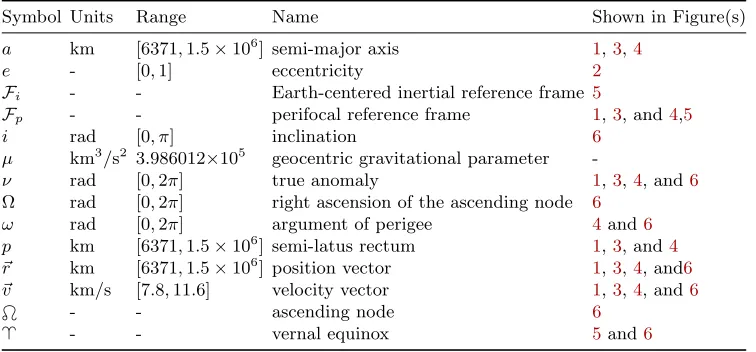
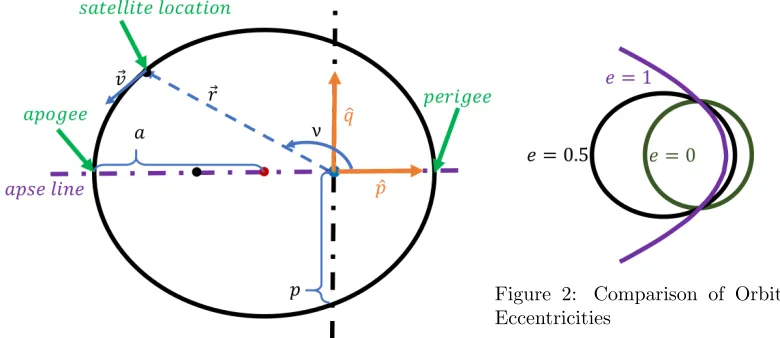
Spacecraft motion may generally be described by conic sections (circles, ellipses, parabolas, and hyperbolas). Orbits are modeled as ellipses in a plane with the Earth at one focus, as shown in Figure1. The orbit may be described in a perifocal reference frameFp, which is specific to the orientation of the orbit and centered on the center of the Earth, where ˆpis a unit vector pointing from the center of the Earth to perigee (the shortest distance from the center of Earth to the edge of the ellipse defining the orbit), ˆqis orthogonal within the plane and aligned with the semi-latus rectum, and ˆw is perpendicular to the orbital plane completing the orthogonal set. The perifocal orbit name comes from its use of perigee (“peri”) in defining the first axis and the use of orbital ellipse’s focal point (“focal”) where Earth resides as the origin. The ellipse’s shape is defined by the semi-major axisa, which is the furthest distance from the center of the ellipse to the edge, and eccentricitye, which is a measure of how much the orbit deviates from a circular orbit. As shown in Figure 2, an eccentricity of zero corresponds to a circular orbit and an eccentricity of one corresponds a parabolic trajectory that escapes Earth orbit. The location of the satellite within the elliptical orbit is described by the true anomalyν, which is the angle from the unit vector pointing to perigee ˆpand the position vector~rpointing from the center of the Earth to the satellite, as shown in Figure1. The velocity vector~v of the orbit is tangential to the ellipse at the location of the satellite.
Also specified in the orbital frame is the semi-latus rectum, calculated from the semi-major axisaand eccentricitye, as described by
p=a(1−e2). (1)
The magnitude of the position vector~r, denotedr, which represents the distance from the center of the Earth to the satellite, changes throughout the orbit and is calculated using
r=|~r|= p
Figure 1: Perifocal Orbital Frame
Figure 2: Comparison of Orbit Eccentricities
Within the perifocal frameFp, the evolution of the spacecraft is modeled using Kepler’s law of equal areas
˙ ν =
rµ
p3(1 +ecosν)
2. (3)
In our proposed benchmark, each satellite has a single state variable corresponding to ν, that evolves according to Equation 3. Equations 2 and 3 are essentially equations of one variable, the true anomalyν, because the semi-latus rectum p, eccentricity e, and geocentric gravitational parameterµare assumed constant for the orbit. The position~rpof the spacecraft in the perifocal frameFp is given by
~ rp=
rcosν, rsinν, 0T
. (4)
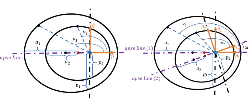
The semi-major axisa, eccentricitye, and true anomaly ν are the first three of six orbital elements. Rather than starting with the full three-dimensional case including all six orbital elements, conjunction prediction algorithms can be evaluated with increasingly more complex combinations of orbits. The case of coaxial and coplanar orbits, as depicted in Figure3, is the simplest model of two spacecraft orbits and may be defined by only three orbital elements: the semi-major axisa, the eccentricity e, and the true anomaly ν. The apse line of each orbit is aligned andν1,ν2are measured from the same line, so the orbits share the same perifocal frame Fp and collisions may be predicted without transforming to a common reference frame.
Even if two satellites are in the same plane, if they do not share the same apse line, the perifocal frames of the orbits are no longer aligned as depicted in Figure4. Therefore, any orbits that are not coaxial and coplanar must be transformed to a common reference frame to compare position vectors and predict collisions. The Earth-Centered Inertial frame provides a convenient common frame for comparisons between orbits and is described in the next subsection.
Figure 3: Coaxial and Coplanar Orbits Figure 4: Noncoaxial, Coplanar Orbits
the three-dimensional orbit that crosses the Earth’s equatorial plan from the southern to the northern hemisphere) to the vector pointing from the center of the Earth to perigee ˆp. The simplest model of two noncoaxial coplanar spacecraft orbits assumes that is the same for both orbits, and only angle between perigee vectors differs (ˆp16= ˆp2) differs byω.
2.2
Orbits in an Inertial Frame
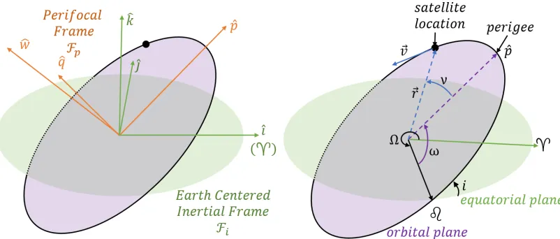
An inertial frame is a reference frame that does not rotate or accelerate and is independent of the satellite’s orbit. The Earth-Centered Inertial (ECI) frame Fi provides a convenient common frame for comparisons between orbits and its usefulness becomes more evident when noncoplanar orbits are compared for conjunction prediction.
The difference between the ECI frameFi and the perifocal frameFp, shown in Figure 5is defined by the argument of perigeeω as previously defined, as well as the orbital inclinationi and right ascension of the ascending node Ω. The inclinationiis the angle from the equatorial plane to the orbital plane at the ascending node. The right ascension of the ascending node Ω is the angle from the vernal equinox(vector from Earth’s center to the Sun when aligned with the equatorial plane on the vernal equinox in the Northern Hemisphere) counter clockwise to the ascending node. These orbital elements are visualized in Figure6. The ECI frame’s ˆiaxis is aligned with the vernal equinox , the ˆj direction is orthogonal to the ˆiaxis so that
together they span Earth’s equatorial plane, and the ˆkaxis is aligned with Earth’s spin axis.
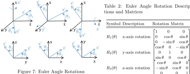
Translating the motion from the inertial frame Fi to the orbital frameFp is accomplished with a rotation matrix Rpi, derived from a sequence of Euler angle rotations. As shown in 7, Euler angles rotations rotate an orthogonal reference frame about one axis, resulting in the rotation matrices in Table2.
Figure 5: Orbital and Inertial Reference Frames
Figure 6: Orbits in the Inertial Frame
the inclination i is 0 because the first and third rotations are about the same axis. Due to the properties of rotation matrices, going from the perifocal frame to the inertial frame is the transpose of the inertial to perifocal frame rotation (Rip =RTpi). The calculation is done with the linear transformation
~ri=Rip~rp= [R3(ω)R1(i)R3(Ω)]T~rp=RT3(Ω)RT1(i)RT3(ω)~rp, (5)
where
Rip =
cΩcω−sΩcisω −cΩsω−sΩcicω sisΩ sΩcω+cΩcisω −sΩsω+cΩcicω −cΩsi
sisω sicω ci
, (6)
andc is an abbreviation for cosine ands is an abbreviation for sine. In inertial frameFi, the x,y, andz components resulting from the rotation matrixRip are
xi= [cΩcω−sΩcisω]xp+ [−cΩsω−sΩcicω]yp+ [sisΩ]zp,
yi= [sΩcω+cΩcisω]xp+ [−sΩsω+cΩcicω]yp+ [−cΩsi]zp, and
zi= [sisω]xp+ [sicω]yp+ [ci]zp.
(7)
3
Satellite Conjunction Verification
x y z x y z x y z y' z' θ1
θ1 θ2 θ2
y'
z
y
θ1 θ1 y'
z' z' z' x' x z θ2 θ2 z'
x' x' θ3 θ3 y' x’ y x
θ3 x'
y'
θ3
Figure 7: Euler Angle Rotations
Table 2: Euler Angle Rotation Descrip-tions and Matrices
Symbol Description Rotation Matrix
R1(θ) x-axis rotation
1 0 0
0 cosθ sinθ 0 −sinθ cosθ
R2(θ) y-axis rotation
cosθ 0 −sinθ
0 1 0
sinθ 0 cosθ
R3(θ) z-axis rotation
cosθ sinθ 0
−sinθ cosθ 0
0 0 1
3.1
Problem Description
The space debris collision detection problem is to prove that no two satellites collide (get within ∆ distance) at any point in time given a list of initial parameters for n satellites and a time bound. We consider the simplest case where satellite parameters are known constants, and the only uncertainty arises from the satellite angle on its orbit, the true anomalyν, which has dynamics defined by Equation3. We want to analyzen-to-ncollision avoidance on thousands satellites, and the proof of safety should be done in dense time. Collisions are considered to occur when two satellites get within some collision radius of each other. For simplicity, we use the infinity norm for this (boxes are used for collision detection).
3.2
Solution Approach
Initially, this problem appears to be ann-dimensional nonlinear system, wherenis the number of orbiting objects, which can be on the order of 1000. Such a system is unlikely to be solved by off-the-shelf reachability methods that can only scale to a dozen or so state variables [8]. In order to analyze this system, we must leverage the problem structure.
Problem Structure. The first type of structure we use is that the dynamics is disjoint.
Satellites move independently of each other when they orbit, and so the state variables do not interact. The derivative of each satellite’sν variable only depends on itself, and no other state variable. This allows us to convert the n-dimensional reachability problem into n one-dimensional reachability problems, and then recombine the reachable sets together after com-putation based on common notions of time [11].
dimensional set, that still contains an infinite number of points. In the case of a 1-d system, however, the boundary of an initial set of states, an interval, is just the lower and upper bounds of the interval. This means that we only need to analyze trajectories from the lower and upper bounds and assure they are safe.
Numerical Simulation. Since we only analyze specific trajectories of a system, we
take a numerical verification approach and assume that numerical simulations can pro-duce accurate system behaviors. Using an off-the-shelf Runge-Kutta numerical simulator (scipy.integrate.RK45), we simulate the lower and upper bounds of ν to predict the time-evolved system states. This also can be used for analyzing intervals of time. Since orbits do not change direction, we can get the range of reachableν values in an interval of time by sampling the endpoints of the range at the start of the time interval and at the end of the time interval, and taking the minimum and maximum over all four values.
Nonlinear Safety Property. A further challenge with this model is that the safety property
is not expressed in terms of ν, but requires converting ν to Cartesianx, y and z coordinates before doing a distance check. This is done according to Equation7, which involves computing sine and cosine ofν as well as some of satellite orbit parameters.
To soundly convert from ranges ofνvalues to ranges ofx, yandzcoordinates, we use interval analysis methods [15]. Other methods, such as Taylor models (or affine arithmetic) could be considered. However, checking for collisions between two Taylor models is more difficult than checking for collisions between two boxes (the result of interval arithmetic), and computing with Taylor models may take more time. In our implementation, the bottleneck was actually the interval arithmetic computation, so we did not experiment with the more complicated methods (although they may allow one to take larger time steps, this could be a direction for future research).
Since we do the conversion using interval arithmetic, the set we use to check for collisions will always be a box, with the property that as theνuncertainty tends towards zero, the volume of the output box will also tend towards zero.
The collision check needs to be done in an n-to-n fashion. We considered three ways to implement this check: exhaustive search, k-d trees, and AABB trees.
The exhaustive search method of conjunction prediction evaluates the distance between every pair of objects. If using an off-the-shelf reachability tool, this is likely the method that would be used. We can take advantage of symmetry in the distance check in order to reduce the number of required checks, but we still expect this method to scale quadratically. The number of required checks with this approach is n(n+1)2 .
However, since we know our problem deals with 3-d spatial coordinates, we can leverage better data structures to reduce the number of checks in the safety condition. The first idea was to use k-d trees. A k-d tree is a binary structure in which the median distance of all points along one axis is determined, grouping the points into those on either side of the median. This process is repeated for each dimension at each level of the tree before being recursively applied, until each level of the tree contains only two points. This enables the tree to be searched relatively quickly for nearest neighbors.
The last idea we considered was using axis-aligned bounding-box (AABB) trees [4]. AABB trees provide a bounding-volume at each inner-node in the tree which that contains the volume of children of that node. They are often used for real-timen-to-n collision detection in video games due to their flexibility and high-performance. Since they do support encoding sets of states, we can insert the reachable regions for each satellite into an AABB tree, and then efficiently check for collisions between sets.
Time-stepping strategy. The last optimization deals with the time-stepping strategy. Since
we want to do analysis with a time bound on the order of days, ideally we would consider large time steps (intervals of time to be analyzed). However, large time steps will lead to large ranges ofνreachable for each satellite, which would leave to large boxes in Cartesian coordinates. This could cause false positives when checking for collisions. Using small time steps, however, would lead to a large number of steps that needs to be analyzed. For this reason, we propose to use a CEGAR-based variable time stepping strategy. We start with a minimum time step such as 0.1 second, and do a step of that size. If the step succeeds (no collisions are detected), we advance time and double the step size. If collisions are detected, we halve the step size and try again without advancing time. If the step size is ever reduced to below the minimum (0.1 seconds), we give up and output that a collision is likely possible.
3.3
Evaluation
We have developed custom code to perform the numerical simulations and leverage the problem structure described in the previous section. The goal was to perform preliminary analysis on the viability of the verification of this benchmark, and we have left a detailed comparison of existing algorithms and tools for nonlinear reachability analysis as a future research item.
In our Python-based implementation, we usescipy’sintegrate.RK45method for satellite simulation, and the pyibex library to perform interval arithmetic. The measurements are performed on an Intel i5-5300U CPU running at 2.30GHz with 16GB main memory. Since the satellite generation is random, the source code used for the benchmark should be included as an attachment with this paper.
We evaluate the proposed approach on two aspects. First, we measure the runtime of various aspects of the algorithm, comparing the previously-described brute force collision check versus the AABB tree method. Next, we analyze the effectiveness of the dynamic time-stepping strategy.
We analyze the system by generating uniformly random satellite parameters. We are concerned with satellites in low-earth orbit, so the satellite height in km, h, is chosen from [6951,7221]. The satellite orbits we are interested are generally round so we use an eccentricity ein the range [0,0.004]. The angles ν, ω, and Ω are all taken from the range [0,2π] andi is taken from the range[0, π].
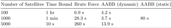
First we compare the brute force search method versus the AABB tree approach. We using a small collision distance of 100 meters (in the infinity norm), with small initialν uncertainty of 0.0001. With these parameters, no collisions should exist in the time frames analyzed.
Table 3: Computation Time Comparison
Number of Satellites Time Bound Brute Force AABB (dynamic) AABB (static)
100 1 hr 6.9 s 4.2 s
1000 1 min 28.3 s 3.7 s 80 s
5000 10 s 260 s 13.9 s
in 3.7 seconds. Finally, with a reach time bound of 10 seconds and 5000 satellites, the brute force method required 260 seconds, whereas the AABB tree approach needed 13.9 seconds. As expected, the AABB method was significantly faster, but still it was still slower than real-time for then= 5000 case.
To analyze the effect of the dynamic time-stepping strategy, we used the AABB method with 1000 satellites for one minute of reach time. A static stepping strategy which always used the minimum step of 0.1 seconds required 80 seconds to complete, compared with 3.7 seconds with the dynamic time stepping approach. In this case, without dynamic times steps, the method runs much slower than real-time. Further, in the dynamic case, the majority of the runtime, 80%, is spent in the interval arithmetic library constructing the boxes of reachable Cartesian coordinates. This means that AABB trees are sufficiently fast so the collision checking is not the bottleneck. The results are summarized in Table3.
Overall, our evaluation shows that reachability analysis, with the enhancements described, can be viable for the space debris collision avoidance problem with a few thousand objects. If we want to scale to tens of thousands or hundreds of thousands of objects, however, further speedups are needed. In the 5000 satellite case, all our current methods were slower than real-time, which is unusable in practice. One idea for speedup would be to consider different time-steps for different objects. Currently, if there is any collision, all objects get rolled back and a smaller time-step is attempted. As we add more objects, the potential for collisions will increase, and so time-step rollbacks will become more common. We will investigate per-object time-steps in future work.
The provided code can be used to create nonlinear benchmarks with any number of dimen-sions. The property is alwaysn-to-ncollision avoidance, but a second parameter is the collision radius in terms of infinity-norm distance. For just evaluating the runtime, a small initial un-certainty in ν, and a small collision radius should be used, so that no collisions occur up to the time bound. To generate instances with collisions, the collision radius and/or the initial uncertainty can be increased.
4
Conclusion
Although we focused on orbital dynamics, many of the problems encountered are more general. Swarm robotics, for example, also have n-to-n collision avoidance requirements. Al-though these system are not 1-dimensional, they do consist of isolated systems that generally fly independently, and so decomposition may still be possible.
References
[1] S. Alfano. Determining satellite close approaches, part 2. Journal of the Astronautical Sciences, 42:143–152, 1994.
[2] K. T. Alfriend, M. R. Akella, J. Frisbee, J. L. Foster, D.-J. Lee, and M. Wilkins. Probability of collision error analysis. Space Debris, 1(1):21–35, 1999.
[3] S. Bak, S. Bogomolov, T. A. Henzinger, T. T. Johnson, and P. Prakash. Scalable static hybridiza-tion methods for analysis of nonlinear systems. InInternational Conference on Hybrid Systems: Computation and Control, 2016.
[4] G. v. d. Bergen. Efficient collision detection of complex deformable models using aabb trees. Journal of Graphics Tools, 2(4):1–13, 1997.
[5] K. Chan. Spacecraft collision probability for long-term encounters.Advances in the Astronautical Sciences, 116(1):767–784, 2003.
[6] N. Chan and S. Mitra. Verifying safety of an autonomous spacecraft rendezvous mission. In G. Frehse and M. Althoff, editors,ARCH17. 4th International Workshop on Applied Verification of Continuous and Hybrid Systems, volume 48 ofEPiC Series in Computing. EasyChair, 2017. [7] X. Chen, E. Abraham, and S. Sankaranarayanan. Taylor model flowpipe construction for
non-linear hybrid systems. Real-Time Systems Symposium, 2012.
[8] X. Chen, M. Althoff, and F. Immler. Arch-comp17 category report: Continuous systems with nonlinear dynamics. In G. Frehse and M. Althoff, editors,ARCH17. 4th International Workshop on Applied Verification of Continuous and Hybrid Systems, volume 48 ofEPiC Series in Computing, pages 160–169. EasyChair, 2017.
[9] T. Dang. Verification et synthese des systemes hybrides. PhD thesis, INPG, oct 2000.
[10] K. J. DeMars, Y. Cheng, and M. K. Jah. Collision probability with gaussian mixture orbit uncertainty. Journal of Guidance, Control, and Dynamics, 37(3):979–985, 2014.
[11] J. Green. Compositional bounded reachability using time partitioning and abstraction, 2012. [12] T. A. Henzinger, P.-H. Ho, and H. Wong-Toi. Algorithmic analysis of nonlinear hybrid systems.
IEEE transactions on automatic control, 43(4):540–554, 1998.
[13] S. A. Hildreth and A. Arnold. Threats to u.s. national security interests in space: Orbital debris mitigation and removal. Technical report, Congressional Research Service, 2014.
[14] B. HomChaudhuri, M. Oishi, M. Shubert, M. Baldwin, and R. S. Erwin. Computing reach-avoid sets for space vehicle docking under continuous thrust. In Decision and Control (CDC), 2016 IEEE 55th Conference on, pages 3312–3318. IEEE, 2016.
[15] L. Jaulin. Applied interval analysis: with examples in parameter and state estimation, robust control and robotics, volume 1. Springer Science & Business Media, 2001.
[16] C. Jewison and R. S. Erwin. A spacecraft benchmark problem for hybrid control and estimation. InDecision and Control (CDC), 2016 IEEE 55th Conference on, pages 3300–3305. IEEE, 2016. [17] T. T. Johnson, J. Green, S. Mitra, R. Dudley, and R. S. Erwin. Satellite rendezvous and
con-junction avoidance: Case studies in verification of nonlinear hybrid systems. In International Symposium on Formal Methods, pages 252–266. Springer, 2012.
[18] R. P. Patera. Space vehicle conflict-avoidance analysis.Journal of guidance, control, and dynamics, 30(2):492–498, 2007.