Multiple quality tests for analysing CO

© Author(s) 2008. This work is distributed under the Creative Commons Attribution 3.0 License.

Multiple quality tests for analysing CO

2

fluxes in a beech temperate

forest

B. Longdoz, P. Gross, and A. Granier

INRA, UMR1137 Ecologie et Ecophysiologie Foresti`ere, Centre de Nancy, F-54280 Champenoux, France Received: 30 August 2007 – Published in Biogeosciences Discuss.: 13 November 2007

Revised: 17 March 2008 – Accepted: 2 April 2008 – Published: 7 May 2008

Abstract. Eddy covariance (EC) measurements are widely used to estimate the amount of carbon sequestrated by ter-restrial biomes. The decision to exclude an EC flux from a database (bad quality records, turbulence regime not ad-equate, footprint problem,. . . ) becomes an important step in the CO2 flux determination procedure. In this paper an

innovative combination of existing assessment tests is used to give a relatively complete evaluation of the net ecosys-tem exchange measurements. For the 2005 full-leaf season at the Hesse site, the percentage of rejected half-hours is rel-atively high (59.7%) especially during night-time (68.9%). This result strengthens the importance of the data gap filling method. The data rejection does not lead to a real improve-ment of the accuracy of the relationship between the CO2

fluxes and the climatic factors especially during the nights. The spatial heterogeneity of the soil respiration (on a site with relatively homogenous vegetation pattern) seems large enough to mask an increase of the goodness of the fit of the ecosystem respiration measurements with a dependence on soil temperature and water content when the tests are used to reject EC data. However, the data rejected present some common characteristics. Their removal lead to an increase in the total amount of CO2respired (24%) and

photosynthe-sised (16%) during the 2005 full-leaf season. Consequently the application of our combination of multiple quality tests is able improve the inter-annual analysis. The systematic application on the large database like the CarboEurope and FLUXNET appears to be necessary.

1 Introduction

Carbon dioxide exchanges between the terrestrial ecosys-tems and the atmosphere are of major importance for

cli-Correspondence to: B. Longdoz ([email protected])

mate change and therefore for the future of the vegetation (Houghton et al., 1998). The quantification of CO2 fluxes

at the ecosystem-atmosphere interface is one of the primor-dial steps to improve our knowledge about the ecosystem carbon budget. The eddy covariance (EC) technique (Aubi-net et al., 2000) provides the opportunity to have a direct measure of these fluxes. Sites equipped with EC systems spread around the world (Baldocchi et al., 2001) with, at the present time, more than 400 stations (http://www-eosdis. ornl.gov/FLUXNET), some of them have been running con-tinuously for more than 10 years. The EC technique is based on high frequency (10–20 Hz) records of wind speed compo-nents, sonic temperature, CO2 and H2O concentrations and

includes a post processing procedure with several method-ological choices (Finnigan et al., 2003). The method re-quires periods with developed atmospheric turbulent regime (Feigenwinter et al., 2004; Rebmann et al., 2005). For ex-ample, during quite nights, the CO2 produced by the

res-piration of the ecosystem components can be stored by the canopy air or blown horizontally by advection (Paw et al., 2000) and is not registered by the EC system. For our temper-ate beech forest site (Hesse, France), some corrections with canopy air storage measurement and selection of the data without advection (Aubinet et al., 2005) are performed but they don’t completely erased all the problems as short-term net CO2flux fluctuations during night-time (Longdoz et al.,

2004) without any biophysical explanation are still observed. The question of the presence of instrumental anomalies, non stationary conditions, footprint outside of our beech forest have then arise to explain these observations. These prob-lems lead to errors and propagation of uncertainties that are able to mask some properties of biophysical processes. The amount of data produced is so large that the visual detection and removing of non adequate data is impossible. The im-provement of the EC dataset quality by automatic procedure has become a real challenge for the EC scientific community (Richardson et al., 2006a; Papale et al., 2006).

Different authors have presented several tests for the se-lection of the EC data (Vickers and Mahrt, 1997; Foken and Wichura, 1996, G¨ockede et al., 2004) and several methods to fill the gaps existing in the dataset (Falge et al., 2001; Hui et al., 2004; Ruppert et al., 2006, Moffat et al., 2007). In this study, we combine most of the tests proposed for the CO2flux. This innovative grouping is applied to the records

from the Hesse site for the full-leaf 2005 season. This period presents some reasonably standard climatic conditions (no extreme events). The duration of the period is short enough to assume relatively stable ecosystem response to environ-mental factors and long enough to provide a sufficient quan-tity of data (even after quality tests selection) to analyse these responses. The impact of our relatively complete combina-tion of tests is evaluated by comparison with the datasets in-cluding or not inin-cluding the records incriminated by the tests. The analysis is performed on the relationships between CO2

fluxes and climatic factors and on the total fluxes accumu-lated during the full-leaf 2005 season.

2 Material and methods

2.1 Site

All the data used in the present analyses come from an ex-perimental plot located in the state forest of Hesse (48◦400N, 7◦040E, North-east of France). This site belongs to the Car-boEurope network. The climate is temperate with 860 mm and 9.3◦C for mean annual rainfall and air temperature (mean on 30 years 1974–2003). The stand is composed mainly (90%) of Beech (Fagus sylvatica). For the period consid-ered in this paper (full-leaf season from 15 May to 14 Octo-ber 2005) the trees were 39 years old and 17 m high (mean value), the LAI (5.1 m2m−2)and tree density (2916 stem/ha) were relatively low compared to the previous years (mean LAI 7.3 m2m−2)because of the thinning performed during the winter 2004–2005. The gentle slope (approximately 3% going down in the Northeast direction) is sufficient to induce advection during the stable nights (Aubinet et al., 2005). The distance between the EC tower and the forest edge varies with wind direction from 390 m to 1610 m. The full-leaf season selected (2005) can be qualified as relatively normal when compared to the mean climate of the 30 previous years. The mean air temperature is slightly lower (16.0–16.4◦C) and even if the total amount of precipitation is higher (381– 241 mm) the cumulative global radiation is also more impor-tant (2957–1846 MJ m−2)for 2005. A more detailed descrip-tion of the site can be found in Granier et al. (2000a, b). 2.2 Flux measurements

The net CO2 fluxes between the ecosystem and the

atmo-sphere (Fc) were measured with an eddy covariance system composed by a sonic anemometer Solent R3 (Gill Instru-ments Ltd, Lymington, UK) and an infrared gas analyser

Li-Cor 6262 (Li-Li-Cor Inc., Lincoln, NE, USA). The anemome-ter measuring the three components of the wind velocity and sonic temperature (u,v,w,T )at 20 Hz is located on a tower at 23.5 m above ground. The IRGA measuring CO2 and

H2O concentrations at 10Hz is located at the ground level,

analysing the air sucked from a sampling point close to the anemometer with an air flow rate of 6 l min−1. A mass flow controller (Model 5850, Brooks, Veenendaal, Netherlands) controls the airflow. The computer acquires the data with the software Eddymeas (Kolle and Rebmann, 2007). To im-proveu,vandwdata, correction for sonic anemometer angle of attack errors is performed (Naka¨ı et al., 2006). This error becomes significant when the wind vector angle to the hori-zontal plane is superior to 20◦(threshold value depending on the sonic anemometer type). It is provoked by transducers self-sheltering or flow distortion induced by the anemometer frame. For each half-hour, the Fc fluxes are calculated from high frequencywand CO2concentration measurements

us-ing block averagus-ing operator (Finnigan et al., 2003) and pla-nar fit as coordinates rotation method (Wilczak et al., 2001). Finally, frequency correction applied to Fc follows the pro-cedure proposed by Aubinet et al. (2000).

The net ecosystem exchange (NEE) is obtained by the summation of Fc and change in CO2storage in the canopy

air (Sc). Sc corresponds to the difference between the to-tal amount of CO2below the eddy covariance measurement

height, at the beginning and the end of the half-hour. This amount of CO2is determined from a profile of concentration

estimated from measurements at 6 different heights (22 m, 10.4 m, 5.2 m, 2 m, 0.7 m, 0.2 m). These measurements are performed with an infrared gas analyser Li-Cor 6262 (Li-Cor Inc., Lincoln, NE). For each level, the concentration used for the Sc computation is the average of the values recorded dur-ing 10 s after purge. More information about tubdur-ing, pumps and filters used are given in Granier et al. (2000b).

2.3 Data check procedure

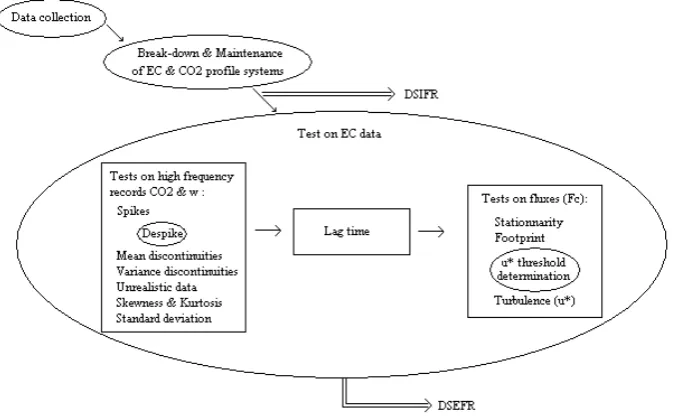
The eddy covariance data treatment used in this study in-cludes several tests (Fig. 1) to detect flux sampling problems, periods with advection, low climatic stationarity or when flux is coming out of the target forest plot. After removal of peri-ods corresponding to break-down and maintenance of the EC and profile systems, the records are first flagged following Vickers and Mahrt (1997). The objective is to identify abnor-malities that may result from instrumental or data recording problems coming from the anemometer or the IRGA (corre-sponding to hard flag in Vickers and Mahrt). For each half-hours, the tests on high frequency measurements of vertical wind velocity and CO2concentration identify first the

Fig. 1.

Fig. 1. General scheme of the data check procedure including the different tests applied on the data belonging to the Data Set

Includ-ing/Excluding Flagged Records (DSIFR/DSEFR).

the half-hour is flagged if one of these parameters is outside of the tolerable range. The criteria to define a spike, an un-realistic value, a discontinuity and a tolerable range for spike percentage, higher-moment statistics and standard deviation are based on threshold values. As proposed by Vickers and Mahrt (1997), the thresholds are empirically adjusted for the Hesse site by inspection of frequency distributions of the pa-rameters tested. The objective is to flag any records with obvious instrument problems. This threshold determination procedure realised for the Hesse 2005 full-leaf season can be illustrated by the choice of upper limit of the tolerable range for the kurtosis of CO2concentration (C)data, which

is the more selective test (see results section). The upper limit of the kurtosis is set to 7.9 to be sure to flag the half-hour record like the one presented in the Fig. 2a. Indeed, the kurtosis of this half-hour is 8.1 because of few irregularities (too large to be considered as spikes) that happen at regu-lar interval indicating their instrumental origins. This half hour record has to be flagged. Moreover, we have not found any half-hour with a lower kurtosis and presenting apparent instrumental problem. For example, turbulence with vary-ing intensity (Fig. 2b) can explain a kurtosis slightly lower than the threshold (7.7) and should not be flagged. After the thresholds set up, the flag procedure is automatic and con-trary to Vickers and Mahrt (1997) all the half-hours flagged have not been individually analysed to verify the origin of the flux-sampling problem. This procedure is not materially feasible when it is applied to large datasets. In consequence it is possible that a few correct fluxes are flagged but this conservative procedure, excluding a maximum of technical anomalies, is preferable.

1 1

Fig. 2a. 2

3

4 5

1 1

Fig. 2b. 2

3 4

Fig. 2. (a) Example of high frequency records of CO2concentration (16 May 18:30 GMT) with instrumental anomalies.

(b) Example of high frequency record of CO2 concentration (18 July 22:00 GMT) with turbulence regime with varying intensity.

The last test to detect instrumental abnormalities is the verification of the airflow rate in the tubing transporting the air from the sampling point (at the top of the tower) to the EC IRGA. This rate is controlled and measured by a mass flow controller (Tylan 261, Tylan Corporation, Torrance, CA, USA). It is set to 6 l min−1 leading to a constant time lag of 4.8 s betweenw andC measurements. The flag is ac-tivated when the airflow rate is 10% below or above the de-sired value. This range is chosen because the post-processing programme is able to correct any deviation of the time lag in this range.

Additionnal tests do not refer to instrumental abnormal-ities. The first one check the Fc stationarity following the procedure presented by Foken and Wichura (1996). The Fc value determined for the half-hour period is compared to the mean out of six 5-min Fc from the same period. The flag is activated when the difference between both values (due for example to changing weather conditions) is above 30% so when the Fc data could not be used for fundamental research (Foken et al., 2004). The second test verifies if the footprint area is located in the targeted ecosystem (young beech plots of the Hesse forest). The Schuepp model (Schuepp et al., 1990) modified by Soegaard et al. (2003) determines the Fc footprint area. The record is flagged when more than 10% of Fc is coming from patches located out of Hesse beech forest. The spatial resolution used corresponds to patches delimited by circles centred on the tower with diameters multiples of 50 m and lines passing by the tower and separated from each others by an 5◦_{angle The forest edge is determined with the}

Hesse land use map already utilized in Rebmann et al. (2005) and Gockede et al. (2007). The last test confirm if the turbu-lent regime is developed enough to applied the EC method (u∗test). Thisu∗has been elaborated because different au-thors (Staebler et al., 2004; Aubinet et al., 2005) have shown that NEE estimated by summation of Fc and Sc can under-estimate CO2exchanges during periods with low turbulence

(low friction velocityu∗). Night-time Reco measurements clearly highlight this underestimation. At constant tempera-ture, Reco drops down whenu∗decreases. This observation has no apparent biophysical explanation. At the Hesse site, additional measurements have proven that some CO2

emit-ted during night by the ecosystem components goes out of the forest by horizontal advection when air mixing is lim-ited (Aubinet et al., 2005). This CO2is not detected by the

eddy covariance or profile concentration measurement sys-tems explaining flux underestimation. We have established a u∗threshold below which Reco is not correctly measured by a two step procedure. In the first step, the temporal variabil-ity of Reco, mainly due to temperature fluctuations, is deter-mined. Using data during periods without water stress and no flagged by the previous tests, the dependence of Reco on temperature is fitted (regression algorithm presented in the following section) by a Q10relationship (Black et al., 1996):

Reco=RecoT ref·Q

T−T ref

10

10 (1)

whereQ10is the parameter reflecting the temperature

sen-sibility and RecoT ref is the Reco value for a reference tem-perature (T ref). Each half-hour Reco is then divided by Q

T−T ref

10

10 to obtain a value Recos that should be relatively

constant during non water stressed periods. The second step consists in distributing Recos inu∗classes. For each class, we compute(Recos)cl corresponding to the Recos class av-erage, and(Recos)hicorresponding to the Recosaveraged on all the data withu∗above the upper limit of the class. The

ob-jective is to detect the classes with a(Recos)cl significantly (p<0.05) lower than(Recos)hi (comparison procedure de-scribed in Sect. 2.5). Among the latter classes, the one with the higheru∗is selected. Theu∗threshold corresponds then to the upper limit of this class.

2.4 Datasets

Two datasets are established both compiling the main mi-crometeorological variables (global radiation, air and soil temperature, photosynthetic photon flux density, soil water content, air humidity, friction velocity. . . ) and the NEE val-ues for the 7344 half-hours between the 15 May and 14 Oc-tober 2005. In the first dataset, the gaps in the NEE corre-spond only to the breakdown and maintenance periods. This dataset is called DSIFR (DataSet Including Flagged Records) in the following (Fig. 1). In the other dataset, in addition, the records flagged by the tests are removed and replaced by gaps (DataSet Excluding Flagged Records, DSEFR, Fig. 1). Two different dataset partitioning are applied during the analysis. The partitioning between night and day is based on global radiation (Rg) with night records corresponding to Rg below 3 Wm−2. During night-time NEE corresponds to ecosystem respiration (Reco) and during daytime to the sum of gross primary productivity (GPP) plus Reco. The second divi-sion aims at isolating the periods without soil water stress for Reco. As soil respiration represents usually the major part of Reco (Law et al., 1999; Longdoz et al., 2000) and be-cause Ngao (2005) has demonstrated that soil respiration in the Hesse forest is limited by water depletion when soil wa-ter content on the first 10 cm (SWC) is below 0.2 m3m−3; we have adopted this threshold for the dataset partitioning. 2.5 Statistical analysis and regression

Table 1. Number of half-hours flagged by the different tests and

fraction to the total 2005 full-leaf period (MFC corresponds to mass flow controller). The values given for the three last tests are com-puted from a dataset where the half-hours flagged by the three first tests on anomalies have been excluded. The total value corresponds to the number of half-hours flagged by at least one test (not equal to the sum because of data flagged by more than one test).

Test Flag

n %

Anemometer anomalies 117 1.6

CO2IRGA anomalies 2297 31.3

MFC anomalies 5 0.1

Stationarity 898 12.2

Footprint 76 1.0

u∗ 903 12.3

Total 4038 55.0

3 Results-discussion

3.1 Tests control results

Among the 7344 half-hours treated, only 2.1% correspond to total breakdown (mainly electricity failure) or maintenance of the EC system and 2.6% to specific maintenance or bad functioning of the profile sampling system. On the remain-ing Fc data (7001 values), flags are activated on 55.0% of the data (4038 half-hours). Consequently, following our pro-cedure 59.7% of the total period is not acceptable in the DSEFR. This is a relatively high percentage but not very sur-prising in regard to the proportion already presented in the literature. Rebmann et al. (2005) flagged 28% of the Hesse Fc for the summer 2000 only with the stationarity test. Even if the flagging procedure is not completely identical, Vick-ers and Mahrt (1997) flagged during their measurement cam-paigns one-third of the records with the variance discontinu-ity test and one-half because of too large kurtosis.

In our procedure, the causes of the Fc flags can be divided in six categories: anemometer, CO2 IRGA and mass flow

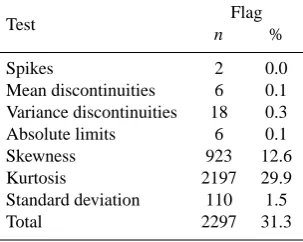
controller malfunctioning, lack of stationarity, too large foot-print and too lowu∗. The percentages of Fc flags due to each category are presented in the Table 1. The values given for the three last tests are computed from a dataset where the half-hours flagged by the three first tests on anomalies have been excluded. Three tests appear to be highly restrictive: CO2 IRGA anomalies,u∗ and stationarity. The percentage

of stationarity flags is lower to that estimated by Rebmann et al. (2005) for the Hesse summer 2000 (28%) but the data were not selected before through the CO2anomalies test as

here. The sum of all the half-hours flagged by the differ-ent tests (4296) exceeds the total value given in the Table 1 (4038) because of multi-flagged data

Table 2. Number of half-hours flagged by the different tests

con-cerning the CO2anomalies and fraction to the total 2005 full-leaf period. The total value corresponds to the number of half-hours flagged by at least one test (not equal to the sum because of data flagged by more than one test).

Test Flag

n %

Spikes 2 0.0

Mean discontinuities 6 0.1

Variance discontinuities 18 0.3

Absolute limits 6 0.1

Skewness 923 12.6

Kurtosis 2197 29.9

Standard deviation 110 1.5

Total 2297 31.3

To go one step further in the analysis and according to the Sect. 2.3, we subdivided the CO2IRGA flag into seven tests:

spikes, mean discontinuity, variance discontinuity, absolute limits, skewness, kurtosis and standard deviation. The higher percentage of bad data is obtained by the kurtosis test (Ta-ble 2) with flags on 29.9% of the total period. This predomi-nance of the flag activation by the kurtosis test has also been observed by Vickers and Mahrt (1997) on their own measure-ments and comes perhaps from the fact that high momeasure-ments values are probably affected by intermittent turbulent regime in addition to instrumental anomalies. As for Table 1, the sum of all the half-hours flagged by the different CO2IRGA

tests (3262) exceeds the total value (2297) because of multi-flagged data. Only two half-hours are multi-flagged by the spike test. Indeed, the sudden variations in the records are often larger than the maximum width of what can be considered as spike (4 points equivalent to 0.4 s). These variations are taken into account in the higher-moment statistics explaining their relatively high percentages of flags.

3.2 Friction velocity thresholds

Before to applied theu∗test, the threshold have to be deter-mined (see Sect. 2.3.). Theu∗test will be used to exclude some records only from in DSEFR (Fig. 1) but we have de-termined theu∗threshold for the two datasets to estimate the impact of all other tests presented here (applied before theu∗ one) on this value (for few EC sites theu∗test is used without applying first other tests). Because the Q10 relationship fit

depends on the available dataset, theu∗threshold determina-tion procedure is applied separately on DSIFR and DSEFR. The Q10relationship fit on the Reco data (night NEE) are

per-formed excluding soil water stress periods (Recos represent-ing 17% of the total period). The bin-average is used to erase the impact of the Recos values affected by horizontal advec-tion. We tested soil temperatures at 10 and 5 cm depth as

Table 3. Characteristics of the Q10function fit applied on the DataSet Including Flagged Records (DSIFR) and DataSet Excluding Flagged Records (DSEFR) with the bin-average technique. Numbers inside parenthesis are standard errors/confidence interval.

Dataset Independent variable Reco10(µmol m−2s−1) Q10 R2

DSIFR Ts10 3.2 (0.21/0.43) 1.9 (0.26/0.55) 0.55

Ts5 3.4 (0.32/0.67) 1.7 (0.34/0.73) 0.30

DSEFR Ts10 3.6 (0.24/0.50) 1.8 (0.25/0.53) 0.49

Ts5 3.5 (0.30/0.65) 1.9 (0.35/0.74) 0.44

independent variables. The results of these fits are presented in Table 3. The 10 cm depth soil temperature (Ts10)is chosen

because of its better general aptitude to explain the Reco vari-ations. This is probably due its superior ability to take into account the spatial heterogeneity, because the 10 cm depth soil temperature value is an average of six measurements while the 5cm temperature is measured with only one sensor. The(Recos)cl and(Recos)hi (see Sect. 2.3.) are compared for eachu∗ classes (0.02 m s−1width). Among the classes giving a (Recos)cl significantly lower than (Recos)hi, the one with the higheru∗has 0.09 and 0.11 m s−1as lower and upper limits. This result is valid for the two datasets. For DSIFR, the(Recos)cl and(Recos)hiof this class are respec-tively 3.45 and 4.86µmol m−2 s−1 (p-value=0.001). For DSEFR, (Recos)cl and (Recos)hi are 2.85 and 4.21µmol m−2 s−1 (p-value=0.0005). Consequently (see Sect. 2.3.), theu∗threshold is set to 0.11 m s−1for the flag determina-tion in DSEFR. This value fully agrees with the one obtained by Papale et al. (2006) for Hesse 2001 and 2002 while the determination method was different (Reichstein et al., 2005). This result suggests that theu∗ threshold is relatively con-stant with time. The u∗ filter is apply for both night and daytime and reject respectively 31.3% and 9.0% of the half-hours for a total of 12.3% but a part of these half-half-hours were already flagged by an other test. Then, whenu∗filter is the last test employed, it is responsible of an increase of the gap fraction from 50.3% to 59.7% in DSEFR. This increase is especially large for night-time (from 50.9% to 68.9%) illus-trating the presence of advection events.

Even if our conservative way to set the thresholds for the Vickers and Mahrt (1997) instrumental malfunctioning tests can be responsible of a slightly overestimation of the per-centage of data removed in DSEFR, it’s high value, espe-cially during night-time (68.9%), stresses the importance of the data gap filling method (Moffat et al., 2007).

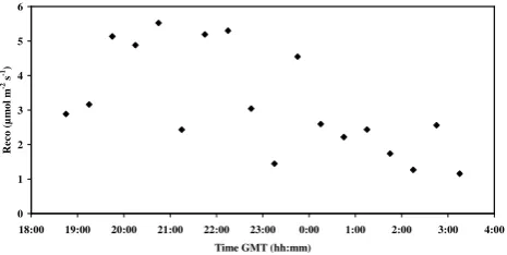
3.3 Temporal variability of ecosystem respiration

The temporal variability of Reco is usually attributed to tem-perature and soil water content variation (Carlyle and Ba Than, 1988; Richardson et al., 2006b). To separate the in-fluence of these two environmental factors, the periods with-out any soil water stress (Sect. 2.4) are selected to analyse

1 Fig. 3.

1

2 0 1 2 3 4 5 6

18:00 19:00 20:00 21:00 22:00 23:00 0:00 1:00 2:00 3:00 4:00

Time GMT (hh:mm)

R

ec

o

(

µ

m

o

l

m

-2 s -1)

Fig. 3. Time evolution of Reco (with short-term fluctuations) during

the night-time between the 5 and 6 August.

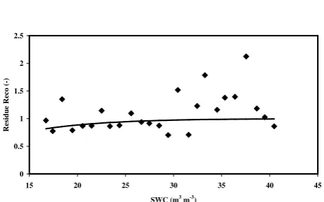
the temperature effect with a Q10 function. The regression

is performed with Ts10as explained above. After computing

the residues of this regression on all the Reco values, they are used to simulate SWC impact with a Gompertz function (Janssens et al., 2003) :

f (SW C)=exp(−exp(a−b·SW C)) f (SW C)=

exp(−exp(a−b·SW C)) (2)

wherea andb are two parameters. The Reco complete function (multiplication of the Q10and Gompertz functions)

is compared to the data to indicate the degree of temporal variability explained by Ts10 and SWC. When this

proce-dure is applied on the DSIFR and DSEFR half-hour data, the determination coefficients (r2)are very low (respectively <0.01 and 0.02). This can reflect the fact that Q10 and

Gompertz functions are not the perfect parameterisation to simulate ecosystem respiration but this explanation is not sufficient to justify so low r2. The other possibility is the existence of factors different from Ts10 and SWC as major

Table 4. Characteristics of the Q10and Gompertz functions fit applied (with bin-average technique) on DataSet Including Flagged Records (DSIFR) and DataSet Excluding Flagged Records (DSEFR). Numbers inside parenthesis are standard errors/confidence interval.

Function Dataset Reco10(µmol m−2s−1) Q10 R2

Q10

DSIFR 3.2 (0.21/0.43) 1.9 (0.26/0.55) 0.55

DSEFR 4.2 (0.31/0.65) 1.8 (0.28/0.58) 0.45

– – a b R2

Gompertz DSIFR 1.7 (2.65/5.47) 19.0 (14.3/29.6) 0.23

DSEFR 0.93 (3.2/6.59) 15.1 (16.8/34.8) 0.12

1 Fig. 4.

1

0 1 2 3 4 5 6 7 8 9 10

9 10 11 12 13 14 15 16 17 18 19 20 21

Ts10 (°C)

R

ec

o

(

µ

m

o

l

m

-2 s -1)

2

Fig. 4. Reco dependence on soil temperature at 10 cm depth. The

dots correspond to the bin-averaged measurements for DSEFR and the line to the fit with a Q10function.

a noteworthy ecosystem spatial heterogeneity and it is not apparently the case for the Hesse site that has a reason-ably homogenous vegetation type and age. To give some indications about the possible impact of footprint changes on Reco temporal variability, we select measurements for a narrow range of Ts10 (from 11.5◦C to 12.5◦C) and

ex-cluding soil water stress period. These measurements are compared according to their provenance from a geograph-ical sector. This comparison cannot completely replace a full analysis combining footprint model and detailed map of soil respiration but this map is not yet available. More-over, the subdivision in patches with homogeneous soil res-piration that would result from this procedure will proba-bly lead, in the DSEFR case, to a too low number of data per patch to investigate the temperature and soil water im-pact for many patches. Our Reco comparison between the geographical sectors shows differences. The more evident one appears when the East-Southeast sector (wind direction between 75◦ and 155◦) is compared to the sector includ-ing the other wind directions. The ecosystem in the East-Southeast sector (mean Reco=6.01µmol m−2s−1)produces significantly more CO2(p=0.034) than the ecosystem out of

this zone (mean Reco=3.99µmol m−2 s−1). When sectors with 45◦width are determined, the ANOVA performed on 5 groups (not enough data between 225◦−360◦) gives a

statis-1 Fig. 5.

1

0 0.5 1 1.5 2 2.5

15 20 25 30 35 40 45

SWC (m3 _m-3₎

R

e

si

d

u

e

R

e

c

o

(

-)

2 3

Fig. 5. Influence of the soil water content (first 10 cm depth) on

the residues of the relationship between Reco and Ts₁₀. The dots correspond to the bin-averaged measurements for DSEFR and the line to the fit with a Gompertz function.

tically significant difference between the 5 means (p=0.029). The large Reco disparity found with this ANOVA (up to al-most 4µmol m−2s−1)has a sufficient order of magnitude to potentially explain many of the short-term Reco variations. One of the possible causes of this heterogeneity could be the soil respiration dependence on carbon to nitrogen content ra-tio (C/N). Ngao (2005) has demonstrated this dependence but it could be completely incriminated if the soil C/N map (work in progress) shows a spatial heterogeneity in agreement with the results of the geographical sectors analysis.

To overcome the spatial heterogeneity problem in the study of the Ts10 and SWC influences on Reco, we use

the bin-average technique. The bin-averaged Q10 (with T ref=10◦C) and Gompertz regressions are presented in Figs. 4 and 5. Bin-average improves clearly the goodness of fit (Table 4) with Ts10being the main explaining factor for

Reco temporal varibility, as usually found (Richardson et al., 2006b). Reco10 (Table 4) are higher than the value for the

equivalent parameter found for soil respiration, as expected (Rs10from 1.5 to 2.4µmol m−2s−1, Ngao, 2005) because of

the leaves and aerial wood CO2production. However, Rs10

represents 65% to 36% of the CO2sources according to the

soil plot investigated. The percentage for the less productive soil plots are low compared to the mean European forests

Table 5. Characteristics of the Michaelis-Menten function fit applied (with bin-average technique) on DataSet Includ-ing Flagged Records (DSIFR) and DataSet ExcludInclud-ing Flagged Records (DSEFR). Numbers inside parenthesis are standard er-rors/confidence interval.

Dataset α GPP2000 R2

DSIFR –0.052 (0.0022/0.0045) –22.8 (0.33/0.67) 0.99 DSEFR –0.072 (0.0053/0.0112) –24.7 (0.43/0.91) 0.98

value (69%, Janssens et al., 2001) but there are perhaps not representative of fluxes measured by the EC system. Con-trary to Reco10, theQ10value is lower in our study (Table 4)

compared to theQ10 estimated for soil (2.55, Ngao, 2005).

This is coherent with the contribution of aerial biomass to Reco that includes sources less sensible to Ts10than the soil.

The tests filtering does not lead to an increase of the coef-ficient of determination (it’s even a decrease) of the regres-sions (for the bin-average and simple cases). The moderate validity of the relationships to describe the ecosystem res-piration and fill the night gaps in the database implies that any overestimation of data rejection rate during night could lead to an increase of the uncertainty of the Reco (and then N EE) seasonal or annual estimation. In this context, the use of theu∗ filter to detect advection events could perhaps be improved (Aubinet et al., 2005; Ruppert et al., 2006). Nev-ertheless, the fact that the regression curves for DSIFR and DSEFR give differences in Reco that range from 19.8% to 34.4% in the 5◦C–20◦C Ts10 interval, proves that the data

eliminated by this filtering are not evenly distributed. 3.4 Temporal variability of gross primary productivity and

net ecosystem exchange

In the two datasets, the GPP is calculated for daytime half-hours showing valid NEE measurements (91% for DSIFR and 46.7% for DSEFR). For each time step, the Reco sim-ulated with the parameterisation presented in the previous section is subtracted from the NEE measurement to achieve GPP. The existence of two Reco parameter sets (DSIFR and DSEFR) leads to two GPP time series. The main factor influencing GPP is the photosynthetic photon flux density (PPFD, µmol m−2 s−1). This influence is parameterised with the Michaelis–Menten relationship adapted by Falge et al., (2001):

GP P= α·P P F D

1−P P F D

2000 + α·P P F D GP P2000

GP P=α·P P F D

1 −

P P F D 2000 +

α·P P F D GP P2000

(3) whereαis the ecosystem quantum yield (µmol m−2s−1) and GPP2000(µmol m−2s−1)is the GPP for PPFD equals to

1 Fig. 6.

1

-30 -25 -20 -15 -10 -5 0

0 200 400 600 800 1000 1200 1400 1600 1800 2000

PPFD (µmol m-2 s-1)

G

P

P

(

µ

m

o

l

m

-2 s -1)

2 3

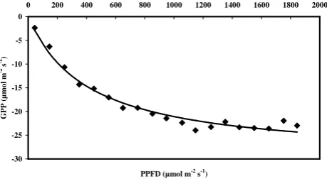
Fig. 6. GPP dependence on photosynthetic photon flux density. The

dots correspond to the bin-averaged measurements for DSEFR and the line to the fit with a Michaelis-Menten function.

2000µmol m−2s−1. Ther2of the regression of this relation-ship on half-hours data are 0.57 (DSIFR) and 0.52 (DSEFR), thus much higher than the Reco-Ts10 ones in the same

con-ditions (<0.01 and 0.02). The lower dispersion of the exper-imental points around the parameterisation curve is probably due to the lower spatial variability for GPP comparing to soil respiration. This comes from the lower spatial variability in vegetation characteristics comparing to the soil ones. To im-prove the GPP-PPFD relationship, the bin-average method is also implemented. This allows hiding spatial variability and possible control of other environmental factors like air temperature (Ta) or vapour pressure deficit (VPD). The influ-ence of GPP-PPFD appears then extremely clearly (Fig. 6, Table 5). The residues of this parameterisation don’t show any dependence on Ta or VPD. This is not surprising in view of the full-leaf 2005 season climate (relatively humid and temperate). Like for Reco, the data selection with the assess-ment tests do not improve the quality of the regression. This is demonstrated by the a DSEFRr2 lower than the DSIFR one (Table 5). However, the difference between the param-eters obtained with these regressions gives significant vari-ation in GPP between DSIFR and DSEFR cases whatever PPFD. The difference ranges from 7.0 to 38.3% when PPFD vary from 2050 to 0µmol m−2s−1. This result suggests that the data eliminated by the filtering possess a common fea-ture.

3.5 TotalReco, GP P andN EE

the DSEFR were filled with the parameter set of DSIFR. The rest of the increase is instigated by the change of the param-eter sets when the DSEFR are chosen. A Similar analysis was performed for the GPP. The GPP generated by DSIFR and DSEFR are respectively –1246.7 and –1440.6 gC m−2, therefore they let to an assimilation increase of 193.9 gC m−2 (15.6%). However, the impact of the environmental factors is larger (27.3%, 52.9 gC m−2). For NEE, the tests induce a sequestration rise of 35.8 gC m−2(6.1%). Comparing to the results for GPP and Reco, the effect of the environmen-tal factors is higher (98.2%,) because this effect is cumulative when GPP is added to Reco to obtain NEE in opposition with the part induced by the choice of the parameter sets (DSIFR or DSEFR).

It is important to note that the impact of the quality tests on the different CO2fluxes have the same order of magnitude

than the expected year to year NEE and especially Reco, and GPP variations with regards to the value already published for forests under similar climate (Aubinet et al., 2002; Car-rara et al., 2003). Therefore, application of the quality tests is able to strongly influence the inter-annual analysis. This conclusion is still valid even if we do not take into account the data gap filling method, considering that a NEE variation of 38.7 gC m−2are only a result from the gap characteristics.

4 Conclusions

The different tests presented in this paper are rarely applied, together and systematically, on large datasets. The results for the 2005 Hesse full-leaf season give an overview of their possible contribution. The high percentage of flagged data detected strengthens the importance to continue the work on data selection and data gap filling methods, especially dur-ing night. The strict data selection does not modify theu∗ threshold.

One of the expected contributions of the quality tests was the reduction of the unexplained short-term Reco fluctua-tions. This was not achieve because of the large spatial het-erogeneity of Reco. Even for a site with homogeneous vege-tation like Hesse, the Reco temporal variation analysis should probably be studied from the respiration spatial heterogene-ity point of view, before focusing on the data qualheterogene-ity. In this context, the way to proceed seems to first apply a footprint model combined with a soil respiration map before to select the data and study the inter-annual variability.

Apparently, the tests have an impact on the dataset prop-erties. On the one hand, the data elimination changes the relationship between the CO2fluxes and the environmental

factors. On the other hand, the general features of the gaps differ when the quality tests are applied. Consequently, the gap filling by the parameterisations, using the environmen-tal factors as independent variables, produce different Reco and GPP values for DSIFR and DSEFR. Even if this con-clusion should be confirm with other parameterizations or

model, the total Reco, GPP and NEE for the 2005 full-leaf season vary by respectively 24, 16 and 6%, with more impor-tant GPP, more CO2produced by respiration processes and

higher net sequestration when tests are applied. The combi-nation of these tests have the potential ability to influence the inter-annual analysis for the CO2fluxes. Their systematic

ap-plication on large databases like from the CarboEurope and FLUXNET experiments seems necessary.

Acknowledgements. This work is founded by the project

Carboeu-ropeIP (GOCE-CT2003-505572) of the European Community and by the GIP Ecofor (French Ministry for Environment).

Edited by: J. Kesselmeier

References

Aubinet, M., Grelle, A., Ibrom, A., Rannik, ¨U., Moncrieff, J., Fo-ken, T., Kowalski, A., Martin, P. H., Berbigier, P., Bernhofer, C., Clement, R., Elbers, J. A., Granier, A., Grunwald, T., Morgen-stern, K., Pilegaard, K., Rebmann, C., Snijders,W., Valentini, R., and Vesala, T.: Estimates of the Annual Net Carbon and Water Exchange of Forest: The EUROFLUX Methodology, Adv. Ecol. Res., 30, 114–173, 2000.

Aubinet, M., Heinesch, B., and Longdoz, B.: Estimation of the car-bon sequestration by a heterogeneous forest: night flux correc-tion heterogeneity of the site and inter-annual variability, Glob. Change Biol., 8, 1053–1071, 2002.

Aubinet, M., Berbigier, P., Bernhofer, C., Cescatti, A., Feigenwin-ter, C., Granier, A., Gr¨unwald, T., Havrankova, K., Heinesch, B., Longdoz, B., Marcolla, B., Montagnani, L., and Sedlak, P.: Comparing CO₂storage and advection conditions at night at dif-ferent CarboEuroflux sites, Bound.-Lay. Meteorol., 116, 63–94, 2005.

Baldocchi, D., Falge, E., Gu, L., Olson, R., Hollinger, D., Running, S., Anthoni, P., Bernhofer, C., Davis, K., Evans, R., Fuentes, J., Goldstein, A., Katul, G., Law, B., Lee, X., Malhi, Y., Meyers, T., Munger, W., Oechel, W., Paw, K. T., Pilegaard, K., Schmid, H. P., Valentini, R., Verma, S., Vesala, T., Wilson, K., and Wofsy, S.: FLUXNET: A New Tool to Study the Temporal and Spa-tial Variability of Ecosystem-Scale Carbon Dioxide, Water Va-por, and Energy Flux Densities, Bull. Am. Meteorol. Soc., 82, 2415–2434, 2001.

Black, T. A., Den Hartog, G., Neumann, H.H., Blanken, P. D., Yang, P. C., Russell, C., Nesic, Z., Lee, X., Chen, S. G., Staebler, R., and Novak, M. D.: Annual cycles of water vapour and carbon dioxide fluxes in and above a boreal aspen forest, Glob. Change Biol., 2, 219–229, 1996.

Carlyle, J. C. and Ba Than, U.: Abiotic controls of soil respiration beneath an eighteen-year-old Pinus radiata stand in south-eastern Australia, J. Ecol. 76, 654–662, 1988.

Carrara, A., Kowalski, A. S., Neirynck, J., Janssens I. A., Curiel Yuste, J., and Ceulemans, R.: Net ecosystem CO2exchange of mixed forest in Belgium over 5 years, Agricultural and Forest Meteorology 119, 209–227, 2003.

Falge, E., Baldocchi, D., Olson, R., Anthoni, P., Aubinet, M., Bern-hofer, C., Burba, G., Ceulemans, R., Clement, R., Dolman, H., Granier, A., Gross, P., Grunwald, T., Hollinger, D., Jensen, N.

O., Katul, G., Keronen, P., Kowalski, A., Lai, C. T., Law, B. E., Meyers, T., Moncrieff, H., Moors, E., Munger, J. W., Pilegaard, K., Rannik, U., Rebmann, C., Suyker, A., Tenhunen, J., Tu, K., Verma, S., Vesala, T., Wilson, K., and Wofsy, S. C.: Gap filling strategies for defensible annual sums of net ecosystem exchange, Agric. For. Meteorol. 107, 43–69, 2001.

Feigenwinter, C., Bernhofer, C., and Vogt, R.: The influence of advection on the short term CO2budget in and above a forest canopy, Boundary-Layer Meteorol., 113, 201–224, 2004. Finnigan, J.J., Clements, R., Malhi, Y., Leuning, R., and Cleugh,

H.: A re-evaluation of long-term flux measurement techniques. Part I: averaging and coordinate rotation, Bound.-Lay. Meteorol., 107, 1–48, 2003.

Foken, T. and Wichura, B.: Tools for quality assessment of surface-based flux measurements, Agric. For. Meteorol., 78, 83–105, 1996.

Foken, T., G¨ockede, M., Mauder, M., Mahrt, L., Amiro, B., and Munger, W.: Post-field data qualtiy control, in: Handbook of Micrometeorology, editeb by: Lee, X., Massman, W., Law, B. E., Kluwer, Dordrecht, 181–208, 2004.

G¨ockede, M., Rebmann, C., and Foken, T.: Use of footprint mod-elling for the characterisation of complex meteorological flux measurement sites, Agric Forest Meteorol., 127 (3), 175–188, 2004.

G¨ockede, M., Foken, T., Aubinet, M., Aurela, M., Banza, J., Bern-hofer, C., Bonnefond, J. M., Brunet, Y., Carrara, A., Clement, R., Dellwik, E., Elbers, J., Eugster, W., Fuhrer, J., Granier, A., Gr¨unwald, T., Heinesch, B., Janssens, I. A., Knohl, A., Koeble, R., Laurila, T., Longdoz, B., Manca, G., Marek, M., Markka-nen, T., Mateus, J., Matteucci, G., Mauder, M., Migliavacca, M., Minerbi, S., Moncrieff, J., Montagnani, L., Moors, E., Ourcival, J.-M., Papale, D., Pereira, J., Pilegaard, K., Pita, G., Rambal, S., Rebmann, C., Rodrigues, A., Rotenberg, E., Sanz, M. J., Sed-lak, P., Seufert, G., Siebicke, L., Soussana, J. F., Valentini, R., Vesala, T., Verbeeck, H., and Yakir, D.: Quality control of Car-boEurope flux data - Part 1: Coupling footprint analyses with flux data quality assessment to evaluate sites in forest ecosys-tems, Biogeosciences, 5, 433–450, 2008,

http://www.biogeosciences.net/5/433/2008/.

Granier, A., Biron, P., and Lemoine, D.: Water balance, transpi-ration and canopy conductance in two beech stands, Agric. For. Meteorol. 100, 291–308, 2000a.

Granier, A., Ceschia, E., Damesin, C., Dufrˆene, E., Epron, D., Gross, P., Lebaube, S., Ledantec, V., Le Goff, N., Lemoine, D., Lucot, E., Ottorini, J. M., Pontailler, J. Y., and Saugier, B.: The carbon balance of a young beech forest, Funct. Ecol., 14, 312– 325, 2000b.

Houghton, R. A., Davidson, E. A., and Woodwell, G. M.: Missing sinks, feedbacks, and understanding the role of terrestrial ecosys-tems in the global carbon balance, Glob. Biogeochem. Cy. 12, 25–34, 1998.

Hui, D. F., Wan, S. Q., Su, B., Katul, G., Monson, R., and Luo, Y. Q.: Gap-filling missing data in eddy covariance measurements using multiple imputation (MI) for annual estimations, Agric. For. Meteorol., 121, 93–111, 2004..

Janssens, I. A., Lankreijer, H., Matteucci, G., Kowalski, A. S., Buchmann, N., Epron, D., Pilegaard, K., Kutsch, W., Long-doz, B., Grunwald, T., Montagnani, L., Dore, S., Rebmann, C., Moors, E. J., Grelle A., Rannik, U., Morgenstern, K., Oltchev,

S., Clement, R., Gudmundsson, J., Minerbi, S., Berbigier, P., Ibrom, A., Moncrieff, J., Aubinet, M., Bernhofer, C., Jensen, N. O., Vesala, T., Granier, A., Schulze, E. D., Lindroth, A., Dolman, A. J., Jarvis, P. G., Ceulemans, R., and Valentini R.: Productiv-ity overshadows temperature in determining soil and ecosystem respiration across European forests, Glob. Change Biol., 7(3), 269–278, 2001.

Janssens, I. A., Dore, S., Epron, D., Lankreijer, H., Buchmann, N., Longdoz, B., Brossaud, J., and Montagnani, L.: Climatic influ-ences on seasonal and spatial differinflu-ences in soil CO₂efflux, in: Fluxes of Carbon, edited by: R. Valentini, Water and Energy of European Forests, Springer-Verlag, Berlin, 235–253, 2003. Kolle, O. and Rebmann, C.: Eddysoft – Documentation of a

Soft-ware Package to Acquire and Process Eddy Covariance Data, Technical Reports – Max-Planck-Institut f¨ur Biogeochemie 10, 88, 2007.

Law, B. E., Ryan, M. G., and Anthoni, P. M.: Seasonal and annual respiration of a ponderosa pine ecosystem, Glob. Change Biol., 5, 169–182, 1999.

Longdoz, B., Aubinet, M., and Franois, L. M.: Model of forest carbon sequestration incorporating aerial wood radiative budget, Agric. For. Meteorol., 125, 83–104, 2004.

Longdoz, B., Yernaux, M., and Aubinet, M.: Soil CO2efflux mea-surements in a mixed forest: impact of chamber disturbances, spatial variability and seasonal evolution, Glob. Change Biol., 6, 907–917, 2000.

Moffat, A. M., Papale, D., Reichstein, M., Hollinger, D. Y., Richardson, A. D., Barr, A. G., Beckstein, C., Braswell, B. H., Churkina, G., Desai, A. R., Falge, E., Gove, J. H., Heimann, M., Hui, D., Jarvis, A. J., Kattge J., Noormets, A., and Stauch, V. J.: Comprehensive comparison of gap-filling techniques for eddy covariance net carbon fluxes, Agric. For. Meteorol., 147 (3–4), 209–232, 2007

Murtaugh, P. A.: Simplicity and complexity in ecological data anal-ysis, Ecology, 88 (1), 56–62, 2007.

Nakai, T., van der Molen, M. K., Gash, J. H. C., and Kodama, Y.: Correction of sonic anemometer angle of attack errors, Agricul-tural and Forest Meteorology, 136, 19–30, 2006.

Ngao, J.: Determinism of ecosystem respiration in a beech forest, Ph.D. Thesis, University Henri Poincar´e Nancy I, 2005. Papale, D., Reichstein, M., Aubinet, M., Canfora, E., Bernhofer, C.,

Kutsch, W., Longdoz, B., S. Rambal, Valentini, R., Vesala, T., and Yakir D.: Towards a standardized processing of Net Ecosys-tem Exchange measured with eddy covariance technique: algo-rithms and uncertainty estimation, Biogeosciences, 3, 571–583, 2006,

http://www.biogeosciences.net/3/571/2006/.

Paw U. K. T., Baldocchi, D. D., Meyers, T. P., and Wilson, K. B.: Correction of eddy-covariance measurements incorporating both advective effects and density fluxes, Bound.-Lay. Meteorol., 97, 487–511, 2000.

ap-plied on eddy covariance measurements at complex forest sites using footprint modelling, Theor. Appl. Climatol., 80, 121–141, 2005.

Reichstein, M., Falge, E., Baldocchi, D., Papale, D., Aubinet, M., Berbigier, P., Bernhofer, C., Buchmann, N., Gilmanov, T., Granier, A., Gr¨unwald, T., Havr’ankov’a, K., Ilvesniemi, H., Janous, D., Knohl, A., Laurila, T., Lohila, A., Loustau, D., Mat-teucci, G., Meyers, T., Miglietta, F., Ourcival, J.-M., Pumpanen, J., Rambal, S., Rotenberg, E., Sanz, M., Tenhunen, J., Seufert, G., Vaccari, F., Vesala, T., Yakir, D., and Valentini, R.: On the separation of net ecosystem exchange into assimilation and ecosystem respiration: review and improved algorithm, Glob. Change Biol., 11, 1424–1439, 2005.

Richardson, A. D., Hollinger, D. Y., Burba, G. G., Davis, K. J., Flanagan, L. B., Katul, G. G., William Munger, J., Ricciuto, D. M., Stoy, P. C., Suyker, A. E., Verma, S. B., and Wofsy, S. C.: A multi-site analysis of random error in tower-based measurements of carbon and energy fluxes, Agric. Forest Meteorol., 136, 1–18, 2006a.

Richardson, A. D., Braswell, B. H., Hollinger, D. Y., Burman, P., Davidson, E. A., Evans, R. S., Flanagan, L. B., Munger, J. W., Savage, K., Urbanski, S. P., and Wofsy, S. C.: Comparing sim-ple respiration models for eddy flux and dynamic chamber data, Agric. Forest Meteorol. 141, 219–234, 2006b.

Ruppert, J., Mauder, M., Thomas, C., and L¨uers, J.: Innovative gap-filling strategy for annual sums of CO2net ecosystem exchange, Agricultural and Forest Meteorology, 138, 5–18, 2006.

Schuepp, P.H., Leclerc, M.Y., MacPherson, J.I., and Desjardins, R.L.: Footprint prediction of scalar fluxes from analytical solu-tions of the diffusion equation, Bound.-Lay. Meteorol., 50, 355– 373, 1990.

Soegaard, H., Jensen, N. O., Boegh, E., Hasager, C. B., Schelde, K., and Thomsen, A.: Carbon dioxide exchange over agricul-tural landscape using eddy correlation and footprint modelling, Agricultural and Forest Meteorology, 114, 153–173, 2003. Staebler, R. M. and Fitzjarrald, D. R.: Observing subcanopy CO₂

advection, Agric. Forest Meteorol., 122, 139–156, 2004. Vickers, D. and Mahrt, L.: Quality control and flux sampling

prob-lems for tower and aircraft data, J. Atmos. Oceanic. Tech., 14, 512–526, 1997.

Wilczak, J. M., Oncley, S. P., and Stage, S. A.: Sonic anemometer tilt correction algorithms, Bound.-Lay. Meteorol., 99, 127–150, 2001.