Linking big models to big data: efﬁcient ecosystem model calibration through Bayesian model emulation

(1)

https://doi.org/10.5194/bg-15-5801-2018 © Author(s) 2018. This work is distributed under the Creative Commons Attribution 4.0 License.

Linking big models to big data: efficient ecosystem model

calibration through Bayesian model emulation

Istem Fer1, Ryan Kelly2, Paul R. Moorcroft3, Andrew D. Richardson4,5, Elizabeth M. Cowdery1, and Michael C. Dietze1

1_{Department of Earth and Environment, Boston University, Boston, MA 02215, USA} 2_{RK Analytics, Durham, NC 27712, USA}

3_{Department Organismic and Evolutionary Biology, Harvard University, Cambridge, MA 02138, USA}

4_{School of Informatics, Computing and Cyber Systems, Northern Arizona University Flagstaff, AZ 86011, USA} 5_{Center for Ecosystem Science and Society, Northern Arizona University, Flagstaff, AZ 86011, USA}

Correspondence:Istem Fer ([email protected])

Received: 20 February 2018 – Discussion started: 26 February 2018

Revised: 5 September 2018 – Accepted: 6 September 2018 – Published: 4 October 2018

Abstract.Data-model integration plays a critical role in as-sessing and improving our capacity to predict ecosystem dy-namics. Similarly, the ability to attach quantitative statements of uncertainty around model forecasts is crucial for model assessment and interpretation and for setting field research priorities. Bayesian methods provide a rigorous data assimi-lation framework for these applications, especially for prob-lems with multiple data constraints. However, the Markov chain Monte Carlo (MCMC) techniques underlying most Bayesian calibration can be prohibitive for computationally demanding models and large datasets. We employ an alterna-tive method, Bayesian model emulation of sufficient statis-tics, that can approximate the full joint posterior density, is more amenable to parallelization, and provides an estimate of parameter sensitivity. Analysis involved informative pri-ors constructed from a meta-analysis of the primary litera-ture and specification of both model and data uncertainties, and it introduced novel approaches to autocorrelation correc-tions on multiple data streams and emulating the sufficient statistics surface. We report the integration of this method within an ecological workflow management software, Pre-dictive Ecosystem Analyzer (PEcAn), and its application and validation with two process-based terrestrial ecosystem mod-els: SIPNET and ED2. In a test against a synthetic dataset, the emulator was able to retrieve the true parameter values. A comparison of the emulator approach to standard “brute-force” MCMC involving multiple data constraints showed that the emulator method was able to constrain the faster

and simpler SIPNET model’s parameters with comparable performance to the brute-force approach but reduced compu-tation time by more than 2 orders of magnitude. The em-ulator was then applied to calibration of the ED2 model, whose complexity precludes standard (brute-force) Bayesian data assimilation techniques. Both models are constrained af-ter assimilation of the observational data with the emulator method, reducing the uncertainty around their predictions. Performance metrics showed increased agreement between model predictions and data. Our study furthers efforts to-ward reducing model uncertainties, showing that the emula-tor method makes it possible to efficiently calibrate complex models.

1 Introduction

(2)

assimila-5802 I. Fer et al.: Linking big models to big data

tion (PDA), which refers to the calibration of model param-eters through statistical comparisons between models and real-world observations to improve the match between them (Richardson et al., 2010). However, despite having more models and data than ever before, we still have not success-fully reduced the uncertainties in our predictions because of the technical difficulties of linking models and data together (Hartig et al., 2012; Fisher et al., 2014). This is particularly true for regional- and global-scale models, which are com-putationally complex and need to be calibrated against large datasets. Three specific technical challenges that need to be addressed in PDA are multiple data constraints, partitioning of uncertainties, and model complexity.

In Bayesian calibration it is possible to use more than one type of data to simultaneously constrain multiple output vari-ables in a model. Using multiple data constraints is particu-larly helpful because model errors can compensate for each other and single variables often do not provide robust con-straints (Raupach et al., 2005; Williams et al., 2009). How-ever, implementing multiple data constraints is challenging because data are available at different spatial and temporal scales, with large differences in observational uncertainties and data volume among measurement types (MacBean et al., 2017; Keenan et al., 2013). The calibration of model param-eters is sensitive to which data are used, how different data sources are combined, and how uncertainties are accounted for (Richardson et al., 2010; Keenan et al., 2011). As opposed to piecewise evaluation of different parts of the model against different datasets, a Bayesian framework allows the evalu-ation of the whole model at once against all data sources, reflecting the connections between variables and the covari-ances among parameters (Dietze, 2017a).

The Bayesian approach also distinguishes among paramet-ric, model structural, and data uncertainties, which is criti-cal for ecologicriti-cal forecasting. Parameter uncertainty refers to the uncertainty about the true values of the model parameters due to data deficiency and model simplification (McMahon et al., 2009; van Oijen, 2017). As models are simplified rep-resentations of reality, it is often not possible to measure the true value of an ecosystem model parameter precisely in the field, regardless of the measurement errors (van Oijen, 2017). However, measurements can still provide estimates for pa-rameter values that make the model represent the reality bet-ter (van Oijen, 2017). Hence, it is possible to reduce param-eter uncertainty with more measurements, conditioned upon the model structure and the measurement error (van Oijen, 2017; Dietze, 2017a). Therefore, the parameter uncertainty should be reflected by probability distributions and propa-gated into model predictions.

By contrast, process or model structural uncertainty refers to the uncertainty about how to represent ecological pro-cesses in models. As every model is a simplification of re-ality, there will always be underrepresented processes or in-sufficiently modeled interactions in ecological models (van Oijen, 2017; McMahon et al., 2009; Clark, 2005). With more

observations, we can advance our theoretical understanding and better characterize ecological processes, but process un-certainty does not necessarily decrease with more data, the way parameter uncertainty does (Dietze, 2017a; Gupta et al., 2012; Clark, 2005). As process uncertainty is part of our im-perfect models, it is part of the uncertainty associated with the model predictions.

Unlike process and parameter uncertainties, data (observa-tion) uncertainty does not need to be propagated into model predictions. Observation error is a result of the limited pre-cision and accuracy of the measurement instruments; hence, the uncertainty about it is not part of the process that we are trying to model (van Oijen, 2017; McMahon et al., 2009). In Bayesian PDA, observation uncertainty should be treated independently of the deviations of model predictions from data as part of the likelihood for observations to inform model predictions without biases (Dietze, 2017a). For a more in-depth terminology for these concepts in the context of process-based models and Bayesian methods, see the review by van Oijen (2017).

Despite the advantages to the Bayesian paradigm when it comes to estimating parameters for ecosystem models, most of this research remains focused on computationally inexpensive models (such as SIPNET, Sacks et al., 2006; DALEC, Keenan et al., 2011; Lu et al., 2017; FöBAAR, Keenan et al., 2013). This is largely due to the relatively high computational costs of Markov chain Monte Carlo (MCMC) techniques underlying most Bayesian computa-tion. Such techniques can require models to be evaluated 104–107 times, which can be prohibitively expensive for even simple models, let alone complex simulation models that may take hours to days to complete a single evalua-tion. In this aspect, the Markovian nature of MCMC tech-niques, which requires that the computation be performed sequentially, proves to be a fundamental limitation. By con-trast, high-performance computing environments are opti-mized for parallel computation and advances in computing power are increasingly being made in terms of number of processors rather than CPU speed. Thus, it is particularly ad-vantageous to consider techniques that are both parallel in nature and which have substantial “memory” (i.e., they use the results from all previously evaluated parameter sets in proposing new parameters rather than just the previous or last few points).

(3)

[image:3.612.111.483.68.627.2]

(4)

5804 I. Fer et al.: Linking big models to big data

(a.k.a. knots; see black dots in Fig. 1), which we obtain by evaluating the model. Once built, emulators generally take far less time to evaluate than the model itself; therefore the emulator is then used in place of the full model in subsequent analyses, i.e., it could be passed to a MCMC algorithm. In comparison to the 104–107 sequential model runs required for MCMC, far fewer model runs are required to construct the emulator, and these runs can be parallelized, as the de-sign points in parameter space are proposed at the beginning or iteratively in large batches.

Emulators are constructed by interpolating a response sur-face between the knots where the model has been run. Previ-ous studies on emulation of biosphere models mostly focused on emulating the model outputs (Kennedy et al., 2008; Ray et al., 2015; Huang et al., 2016). However, comparing model outputs to “big data” requires emulating a large, nonlinear multivariate output space. Furthermore, for the purpose of model calibration what we are actually interested in is not the output space itself but the mismatch between the model and the data, which can typically be summarized by much lower dimensional statistics (e.g., sum of squares).

Instead of constructing an emulator for the raw model out-put, we adopt the approach of constructing an emulator of the likelihood – the statistical assessment of the probability of the data given a vector of model parameters, which forms the basis for both frequentist and Bayesian inference. Emulat-ing the likelihood has the advantage that likelihood surfaces are generally smooth and univariate (Oakley and Youngman, 2017). A further novel generalization we introduce in this study is to emulate the sufficient statistics of the likelihood that contains all the information to calculate the desired like-lihood rather than the likelike-lihood itself. This facilitates esti-mating the statistical parameters in the likelihood, such as the residual error.

Overall, the goal of this study is to validate the emulator’s performance against brute-force MCMC methods in terms of parameter estimation and assess the trade-offs in clock-time and emulator approximation errors. We first tested the emulator performance with the simplified Photosynthesis and Evapotranspiration (SIPNET) model against a synthetic dataset for which we know the true values. Next, we com-pare both brute force and the emulator for calibrating SIP-NET against data from the AmeriFlux Bartlett Experimental Forest site, a temperate deciduous forest in the northeastern US. Third, we use the emulator technique to calibrate the Ecosystem Demography model (version 2, hereinafter ED2), whose computational demands preclude MCMC calibration. Finally, we evaluate the scaling properties of the emulator method and discuss its potential limitations and future appli-cations.

2 Methods

2.1 Emulator-based calibration

A primary methodological focus of this paper is on the tech-nique of parameter data assimilation using a model emula-tor. The general workflow of the emulator method (Fig. 1) is given in Algorithm 1.

Algorithm 1Emulator workflow

(1) Propose initialNknotsparameter vectors.

(2) Run full model with each parameter vector (parallelizable overNknots).

(3) For each model run (K), compare each dataset to the ap-propriate model output variable (V) and calculate a sufficient statistic (TV ,K) summarizing model error.

(4) Fit a separate Gaussian process (GP_V) model for eachTV to construct a response surface describing how model error varies across parameter space (parallelizable overV).

(5) Perform MCMC using the emulators.

fori=1 toNMCMCdo

(5a) Propose a new vector of process-model parameter val-ues.

(5b) Use GPV to draw both the current and proposedTV with interpolation uncertainty (parallelizable).

(5c) Calculate likelihoods fromT.

(5d) Calculate current and proposed posterior values,Piand

P_i−1.

(5e) Accept or reject according to the Metropolis–Hastings rule,Pi/Pi−1.

(5f) Gibbs update statistical parameters conditional on process-model parameters.

end for

(6) (optional) Refine emulator by proposing new design points,

goto(2).

(5)

the overall design matrix. In the current application, the se-quences for each variable are constructed to be uniform quan-tiles of the prior distributions (see Sect. 2.3), which results in greater sampling in the regions of higher probability and less sampling in the tails for nonuniform prior distributions.

The second step (2) is to evaluate the full model using the proposed parameter vectors, and it is the only step in which we run the full model. As these model runs are indepen-dent of each other, they can be performed in parallel. Next (step 3), a sufficient statistic (T) is calculated by compar-ing each model output to each dataset (Fig. 1). Statistic T is sufficient for the job of estimating the unknown parame-ters “when no other statistic calculated from the same sam-ple provides any additional information” (Fisher, 1922). We treat the deviations of model predictions from data in terms of sufficient statistics (T) instead of the likelihood itself be-cause we want to estimate data-model parameters, such as the residual error, as part of the MCMC. For example, as-sume the residuals are distributed Gaussian. In this case,T for a Gaussian likelihood would be the sum of squared resid-uals, 6(yi−µi)2, wherey is the observation and µis the model prediction.

L= n

Y

i=1

N (yi |µ, τ )= n

Y

i=1 √

τ √

2πexp

₋_{τ (y}

i−µ)2 2

(1)

lnL∝ n 2ln(τ )−

τ 2

n

X

i=1

(yi−µ)2

| {z }

T

(2)

From Eq. (2), if we knowT, we can calculate the likelihood without needing the full dataset and the model outputs. This allows us to not only accept or reject a proposed parameter vector (5e) but also sample the precision parameter,τ, con-ditional on that parameter vector (step 5f). Such aT can be found for other likelihood functions as well.

This approach requires constructing an emulator for each dataset (Step 4) instead of building one emulator on the over-all likelihood surface. For example, if carbon (C) and water (H2O) fluxes are used for constraining the model parame-ters, we need to build one emulator that estimates theTCand another one that estimates TH2O. Then, at each iteration of

the MCMC, we can update the model errors (τC andτH2O)

for each response variable conditional upon the emulatedT. However, both the construction and evaluation of the emula-tor for eachT can be carried out in parallel; therefore, build-ing more than one emulator does not defy the purpose of re-ducing computational costs.

In this study, we fitted a Gaussian process (GP) model as our statistical emulator, using the mlegp (v3.1.4) package in R (Dancik, 2013). GP assumes that the covariance between any set of points in parameter space is multivariate Gaus-sian, and the correlation between points decreases as the dis-tance between them increases (mlegp uses a power exponen-tial autocorrelation function). We chose a GP model as our

emulator because of its desirable properties. First, because GP is an interpolator rather than a smoother it will always pass exactly through the design points. Second, GP allows for the estimation of uncertainties associated with interpola-tion – uncertainty for a GP model will converge smoothly to zero at the design points (knots, Fig. 1). Third, among non-parametric approaches, GP is shown to be the best emulator construction method (Wang et al., 2014). The GP model is essentially the anisotropic multivariate generalization of the Kriging model commonly employed in geostatistics (Sacks et al., 1989). Because we are dealing with a deterministic model, we assume that the variance at a lag of distance zero, known as the nugget in geostatistics, is equal to zero, but this assumption could be relaxed for stochastic models. We do not go into further details of GP modeling, or its comparison to other emulator methods, since both are well documented elsewhere (e.g., Kennedy and O’Hagan, 2001; Rasmussen and Williams, 2006).

Once constructed, we pass the emulator to an adaptive Metropolis–Hastings algorithm (Haario et al., 2001) with block sampling, i.e., proposing new values for all parameters at once (step 5). In the MCMC, we use the GP to estimate T for both the current and the proposed parameter vector at each iteration (5b). GP provides a mean and the variance for the estimated values (hereT) given the parameters. To prop-agate this interpolation uncertainty, it is important to draw theT stochastically from the GP and draw new values for both the current and proposed parameter sets at each itera-tion. Once the process-model parameters are updated accord-ing to the Metropolis ratio of current and proposed posteri-ors, statistical parameters of the likelihood can be updated via Gibbs sampling conditional upon the updated process-model parameters (5f).

To build the emulator, the parameter vectors need not be dependent on one another in a Markovian sense. This is in contrast with traditional optimization and MCMC algo-rithms that only leverage the current vector of parameter val-ues when proposing new parameters. The independence of runs here allows us to efficiently leverage all previous runs, in addition to the model evaluations from this step, to it-eratively refine the emulator (step 6). Itit-eratively proposing additional knots over multiple rounds can be more effective because each round refines our understanding of where the posterior is located in parameter space, allowing new knots to be proposed where they provide the most new informa-tion. In this study, new knots were added by proposing 10 % of the new parameter vectors from the original prior distribu-tion and 90 % from the joint posterior of the previous emula-tor round (via resampling the MCMC samples in between the rounds). Unless otherwise noted, all emulator calibrations in this study were run in three rounds, each with 100 K itera-tions of three MCMC chains, using a total ofp3knots forp parameters.

(6)

(DREAM(ZS)) as it is one of the fastest converging al-gorithms known in the literature (Laloy and Vrugt, 2012). The implementation of DREAM(ZS) was provided by the BayesianTools package (Hartig et al., 2017). These package functions were called within the brute-force data assimila-tion framework of PEcAn (v1.4.10), which is an ecosystem modeling informatics system (LeBauer et al., 2013). The em-ulator framework has also been implemented in PEcAn. Both ecosystem models (see next section) used in this study were coupled to PEcAn and the specific runs reported in this paper are given in Appendix A, Tables A7–A8. All PEcAn code is available on GitHub (https://github.com/PecanProject/pecan, last access: 30 September 2018), and the parameter data assimilation (PDA) modules developed here are accessi-ble via modules/assim.batch and modules/emulator. In addi-tion, a virtual machine version of PEcAn with model inputs and code required to reproduce the present study is avail-able online (http://pecanproject.org, last access: 30 Septem-ber 2018).

2.2 Multi-objective parameterization

We focus on three joint data constraints from Bartlett Exper-imental Forest, NH (Lee et al., 2018; also see Appendix A, “Study site”): net ecosystem exchange (NEE) and latent heat flux (LE) as measured by the eddy-covariance tower, and soil respiration (SoilResp) as sampled within the inventory plots. NEE and LE data were filtered for the low friction ve-locity,u∗, values to eliminate time periods of poor mixing. A conservativeu∗ of 0.40 was selected, which results in an elimination of 76 % of the nighttime data. Flux data were not gap-filled because this results in a model–model com-parison rather than a model–data comcom-parison. The error dis-tribution of flux data is known to be both heteroscedastic, with variance increasing with the magnitude of the flux, and to have a double exponential distribution (Richardson et al., 2006; Lasslop et al., 2008). In previous studies, the error dis-tributions of high flux magnitudes and fluxes averaged over time were also argued to be approximately Gaussian (Lasslop et al., 2008; Richardson et al., 2010). However, as we assim-ilate all flux magnitudes at a half-hourly time step and as the errors of flux data have heavy tails like a Laplacian distribu-tion (i.e., big errors are more common than they would be un-der a Gaussian distribution), we modeled the error distribu-tions of NEE and LE fluxes as an asymmetric heteroscedastic Laplacian distribution:

Fluxdata∼Laplace(Fluxmodel, α0+α1·Fluxmodel) (3)

α1=

αp, if Fluxmodel≥0 αn, otherwise

,

where Laplace(µ,α) refers to the Laplace distribution that models the distribution of absolute differences between model prediction and data. Here we accounted for the fact that flux errors scale differently for positive and negative

fluxes by using different scale parametersαpandαn, respec-tively.

Because NEE and LE data are time series, we cannot treat each residual as independent. To reduce the influence of er-ror autocorrelation on parameter estimation, we correct the likelihoods by inflating the variance terms byN/Neff, where N is the sample size and Neff is an estimate of the effec-tive sample size based on the autocorrelation of the resid-uals. However, estimatingNeff is not straightforward to do within the MCMC because, paradoxically, a poor model pre-diction would end up with higher autocorrelation on the residuals, making theNeffsmaller and the values producing those model outputs more likely. We also cannot calculate the autocorrelation on the data itself because flux data con-tain considerable observation error, making the Neff larger than it should be (i.e., also paradoxically indicating that the data provide more information the larger the observation er-ror). To address these apparent paradoxes we propose a two-step approach to estimating effective sample size. First, the latent unobserved “true” fluxes were estimated via a state-space time series model fitted to the flux data, which allows separation of observation error from process variability (Di-etze, 2017b). So as to not impose external structure on this filtering, we use a random walk process model. Second, the AR(1) autocorrelation coefficient,ρ, was estimated on the latent state time series andNeffwas estimated as

Neff=N (1−ρ)

(1+ρ). (4)

For soil respiration (Rd: data, Rm: model), we assume a Gaussian likelihood with a multiplicative bias,k, and a vari-anceσ_R2, which takes the formRd∼N (k·Rm,σ_R2). The bias term is included to account for the scaling from the dis-crete soil collars to the stand as a whole (van Oijen et al., 2011). This term was also introduced because observed soil chamber fluxes were typically over twice the ecosystem res-piration estimated from the eddy-covariance tower (Phillips et al., 2017). As in previous studies, this parameter is also estimated in the calibration (van Oijen et al., 2011), using a standard lognormal distribution as its prior. While the in-troduction of the bias term makes it impossible for these data to constrain the magnitude of soil carbon fluxes, it does provide information on the shape of the functional response (e.g., temperature dependencies). Due to the coarser time step, small sample size (n=39), and the introduction of the bias term, no additional autocorrelation corrections were ap-plied to the soil respiration data.

2.3 Model information and priors

(7)

col-lected in the tower footprint were used to set initial condi-tions for the models (Table A1). We calibrate the models us-ing data from 2005 and 2006. Both models provide outputs at the same half-hourly time steps as the assimilated flux data. SIPNET is a fast model (∼5.5 s per execution, in this study), which makes it suitable for application of traditional brute-force MCMC methods. In contrast, it takes approximately 6.5 h for ED2 to complete a single run for this 2-year period, which precludes its brute-force calibration.

We targeted both the plant physiological and soil biogeo-chemistry parameters of the models. Unlike SIPNET, it is possible to run ED2 simulations with more than one compet-ing plant functional type (PFT). To reduce the dimensionality of the calibration for ED2, differences among PFTs were as-sumed to vary proportionally to the differences among their priors and a parameter scaling correction factor (SF) was tar-geted by the parameter data assimilation algorithm instead of targeting each parameter per PFT. The SF operates on the prior cumulative density function (CDF) probability space [0,1]. For instance, when the SF for a certain parameter is 0.3, it would correspond to the 30th percentile of the param-eter prior for each PFT.

We generated the priors and estimates for model param-eters based on a hierarchical Bayesian trait meta-analysis using PEcAn’s workflow. Meta-analysis priors were speci-fied by fitting distributions to raw data collected from lit-erature searches, unpublished datasets, or expert knowledge (LeBauer et al., 2013). Direct mapping of previous informa-tion to model parameters allows us to account for the uncer-tainties in measurements derived from the collective weight of a large range of studies rather than arbitrarily choosing values from any one study (LeBauer et al., 2017). The use of literature constraints ensures that the posterior parameter es-timates fall within a biologically plausible range and reduces the problem of equifinality, as parameters that are already well constrained cannot vary much, and thus cannot trade off with poorly constrained parameters. The parametric prior and posterior distributions of the targeted parameters are given in Tables A2 and A5–A6 for SIPNET and ED2, respectively. The scaling factors used for common ED2 PFT parameters all have Beta(1,1)prior distributions.

2.4 Emulator experiments

To test and validate the emulator approach we conducted the following experiments: (1) a test against synthetic data us-ing the emulator with SIPNET, (2) a comparison of emulator and brute-force performances against real-world data using SIPNET, (3) a calibration of ED2 with the emulator using real-world data, and (4) a scaling test with the emulator to evaluate how the actual clock time varies as a number of de-sign points (full model runs) using SIPNET.

Before these experiments, we conducted a predictive un-certainty analysis (for more details on the unun-certainty analy-sis workflow in PEcAn please see LeBauer et al., 2013;

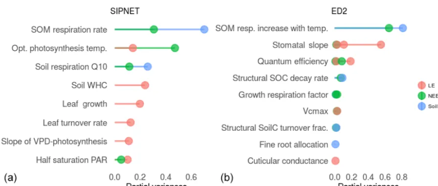
Di-etze et al., 2014) to choose the model parameters for calibra-tion. The parameters that can be constrained by data are those that contribute to the model predictive uncertainty for that corresponding variable. Figure 2 shows the plant physiology and soil biogeochemistry parameters of the models that are targeted by the calibration according to this uncertainty anal-ysis. We chose a cutoff value of 5 % for SIPNET, meaning we only targeted parameters that contribute more than 5 % of the model predictive uncertainty for each variable of interest. In order to facilitate comparisons among the contributions of parameters to predictive uncertainty of output variables with different units, partial variances were used. Partial vari-ances are the varivari-ances of each parameter divided by the sum of variances across all parameters per output variable. For ED2, we lowered this threshold to 1 % because there is more than one PFT that shares the uncertainty. In the end, 9 and 10 parameters were targeted in SIPNET and ED2, respec-tively. To be more specific, the eight (nine) parameters for SIPNET (ED2) that are shown in Fig. 2, plus the multiplica-tive bias parameter, were targeted in the PDA. Therefore, in total 93(103) knots were proposed in three iterative emula-tor rounds (also see Table 1 caption). For ED2, six out of the nine model parameters were plant physiological parameters that are common to all its PFTs, for which we used the scal-ing factors (Fig. A5).

We first tested the emulator performance on retrieving true values using a synthetic dataset. We generated a random pa-rameter set for the SIPNET papa-rameters shown in Fig. 2 and ran the model forward with these values (Table A3). In order to give the synthetic data real characteristics, model outputs were reformatted to have the same gaps, time steps, and sam-ple sizes as the data used in this study. Then, the likelihood parameters were calculated from the synthetic dataset, and next, further noise was added by drawing values from their respective likelihood functions to obtain the final synthetic dataset. In addition, the SoilResp data were multiplied by a constant (k=1.5) to mimic the real world situation. Then, treating the model outputs as a synthetic dataset, we tested whether emulator method posteriors converge on the true val-ues. As this dataset was generated by the model itself, this approach allows us to assume that we have the perfect model (Trudinger et al., 2007; Fox et al., 2009). We compared the emulator run in three rounds to an emulator fit to the same number of knots in a single run to test whether increasing the number of knots iteratively is more effective than proposing the same number of knots in the beginning all at once.

(8)

[image:8.612.75.523.64.254.2]

Figure 2.Results of uncertainty analysis in PEcAn for plant physiological and soil biogeochemistry parameters of SIPNET(a)and ED2(b). The longer the bar the more that parameter contributes to the model predictive uncertainty. The parameters shown above that contribute more than 5 % (1 %) of uncertainty were chosen to target in calibration of SIPNET (ED2) and are shown above.

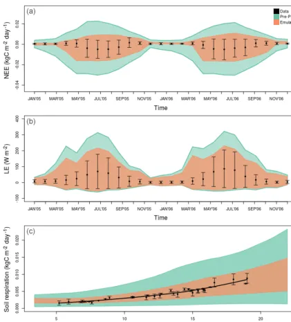
post-calibration performance of ED2. The before- and after-calibration performances of both models were determined by comparing a 500-run model ensemble to data. Ensem-ble runs are forward model runs, with parameter values ran-domly sampled from their distributions (which is the prior distribution for the pre-PDA comparison and the posterior distribution for the post-PDA).

In our scaling experiment, we evaluate the trade-off be-tween the number of model runs and the approximation er-ror by comparing the eight-parameter SIPNET brute-force calibration to emulator calibrations with varying numbers of kknots (k= {120,240,480,960}). To do this, we compared the post-emulator PDA ensemble confidence interval errors relative (RCI) to the post-brute-force PDA ensemble confi-dence interval (CI) in terms of mean Euclidean distance be-tween their 2.5 % and 97.5 % CIs. For each experiment with k different knots and variable (CIE,L,k−CIB,L,k)2, values were calculated where “E” stands for emulator, “B” stands for brute-force ensemble, and “L” stands for the lower CI limit. The same is calculated for the upper CI limit (“U”) and the sum of their mean is used as a score for relative confi-dence interval (RCI) coverage per variable:

RCIVAR,k=mean((CIE,L,k−CIB,L,k)2)

+mean((CIE,U,k−CIB,U,k)2). (5) Next, each RCI vector (RCIVAR= {RCIVAR,960, RCIVAR,480, RCIVAR,240, RCIVAR,120}) is normalized by dividing by its mean to obtain values independent of the units. Then, the sum over the variables (in our case, RCIFINAL=RCINEE+ RCILE+RCISoilResp) given is the final RCI score.

In an additional scaling experiment, we evaluated the ca-pacity to calibrate the model with emulator vs. actual clock time. For this experiment, we chose m parameters (m=

{4,6,8,10}) of SIPNET considering the order of their con-tribution to the overall model predictive uncertainty (Fig. 2, Table A8). For each calibration, we again built an emulator withkknots. After calibration, we used overall deviance of the 500-run ensemble mean as a metric to evaluate calibrated model performances.

3 Results

3.1 Test against synthetic data

The test against synthetic data showed that the emulator was able to successfully retrieve the true parameter values that were used in creating the synthetic dataset (Fig. 3). Diag-nostics showed that the chains mixed well and converged (all visual and Gelman–Rubin MCMC diagnostics can be ac-cessed via the links provided in the workflow ID Table A7). As expected, after each round of emulation, posteriors were resolved more finely around the true values. Especially the multiplicative bias parameter was only able to resolve in the last round (R3). The posteriors of our “all-at-once” test, in which we ran a single emulator proposing all 729 knots at once, compared less well to the true values than the itera-tive approach. This shows that adapitera-tive refinement of the pa-rameter space exploration is more effective than screening the parameter space with the same (cumulative) number of knots.

3.2 Brute-force vs. emulator

(9)

[image:9.612.54.544.62.439.2]

Figure 3.Emulator performance against synthetic data. The red vertical line represents the true parameter values that were used to create the synthetic dataset. Shaded distributions are the posteriors obtained after each emulator round. Dashed lines are the posteriors after a single emulator (all at once, AAO) round built with a total number of knots of all rounds (729 knots) instead of refining the emulator iteratively (first round 243, second round 486, third round 729). All priors were uniform for these parameters, except the multiplicative bias parameter.

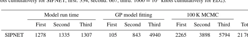
Table 1.Time elapsed (in seconds) for each step of the emulator calibrations. “Model run time” refers to the computation time for running the LHC model ensemble needed to construct the emulator. Sub-columns refer to the rounds of the emulator (first: 243, second: 486, third: 729=93knots cumulatively for SIPNET; first: 334, second: 667, third: 1000=103knots cumulatively for ED2).

Model run time GP model fitting 100 K MCMC

First Second Third First Second Third First Second Third Total

SIPNET 1278 1335 1307 105 843 4940 2265 3898 5794 21 765

ED2 26 018 22 380 22 927 249 2171 7838 2207 4996 7773 96 559

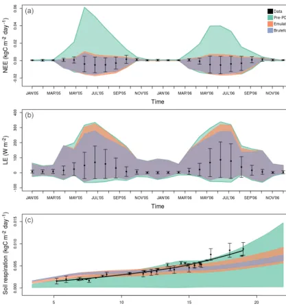
the brute-force approach took 112 h. Both metrics (RMSE and deviance) were improved for NEE and LE after calibra-tion with both methods (Table 2). RMSE for SoilResp got worse after calibration with both methods; however this was expected as we informed the model for the shape of the Soil-Resp flux instead of the absolute magnitude. Indeed, both the deviance metric (which includes the multiplicative bias

[image:9.612.93.504.552.614.2]

(10)

[image:10.612.89.507.66.512.2]

Figure 4.SIPNET performance against real data (black dots) after emulator (orange polygon) vs. brute-force (blue) calibration. The pre-PDA ensemble spread (green) was wider for all variables and was reduced with both methods. Panels(a)and(b)are monthly smoothed time series (for the unsmoothed version please see Fig. A1), while(c)shows the temperature–soil respiration response curve, plotted with a locally weighted scatter plot smoothing (LOESS) line and residuals from a fitted temperature response function as a conservative estimate of the error bars. All polygons show the 2.5 %–97.5 % CI.

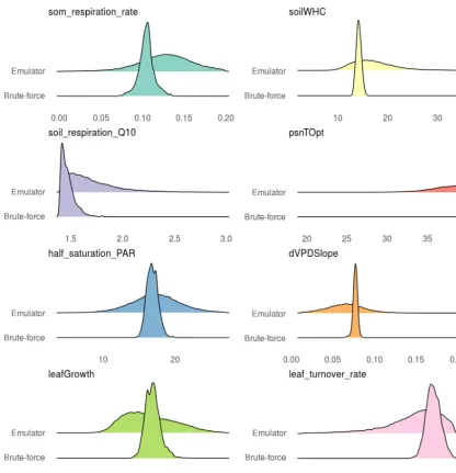
numerical approximation uncertainty in parameter estimates, which propagates into wider confidence intervals in predic-tions. This can also be seen in the posterior distributions in which brute-force has tighter posterior distributions than the emulator (Fig. 5). The strongest correlations between leaf growth and leaf turnover rate, leaf growth and half saturation PAR, soil respiration rate and soil respiration Q10 were also detectable in emulator posteriors (emulator Fig. A3, brute-force Fig. A4).

(11)

[image:11.612.87.504.65.497.2]

Figure 5.Posteriors from the emulator vs. brute-force approaches with SIPNET after calibration against real-world data.

Table 2.Performance statistics of ensemble means before and after the PDA for both models and output variables. While root-mean-square-error (RMSE) scores evaluate the deviations of model predictions from data, deviance (−2×log-likelihood) scores evaluate the goodness of fit under the assumed data model. For both metrics lower scores are better.

NEE LE SoilResp

pre-PDA post-PDA pre-PDA post-PDA pre-PDA post-PDA

RMSE

SIPNETE 140 43 89 79 18 26

SIPNETB 43 77 32

ED2 122 68 124 89 29 18

Deviance

SIPNETE 2745 976 9879 8424 −1333 −1353

SIPNETB 944 8331 −1315

ED2 3152 1523 9914 9103 −1380 −1390

[image:11.612.102.496.570.682.2]

(12)

[image:12.612.87.508.65.529.2]

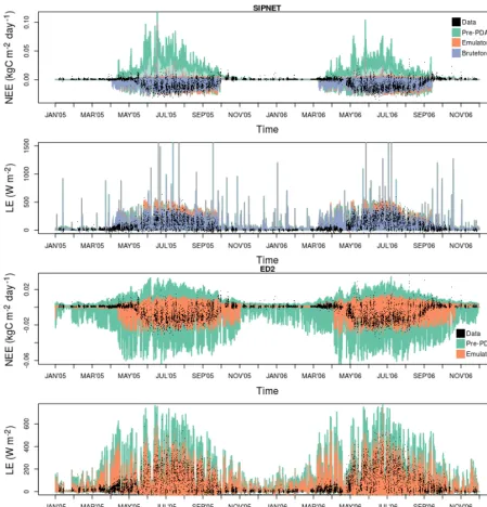
Figure 6.Pre-PDA vs. post-PDA ED2 performance against real-world data. Panels and colors are the same as in Fig. 4.

3.3 ED2 calibration

The emulator calibration for ED2 took ∼27 h (≈96 559 s, Table 1). In contrast, a 100 K iteration of Metropolis– Hastings MCMC with ED2 would have taken approximately 74 years. Both metrics for all variables showed improvement post-PDA (Table 2) and their ensemble spread became nar-rower (Fig. 6). Fitted parametric posterior distributions of ED2 are given in the Appendix (Fig. A5, Table A6). In ad-dition, all raw MCMC samples and posterior density distri-bution plots are available in the respective workflow direc-tories (see Table A7). While all the chains are mixed and

converged, the growth respiration factor and fine root alloca-tion scaling factors were less well resolved, indicating that a fourth round might improve their calibration; however, these model outputs were not too sensitive to these parameters (Fig. 2).

(13)

fluxes (top panels of Figs. 4 and 6). Both pre- and post-PDA ED2 performance for SoilResp was better than SIPNET (bot-tom panels of Figs. 4 and 6). ED2 also captures the summer diurnal cycle better than SIPNET and both models were im-proved after emulator PDA (Fig. A6).

3.4 Emulator scaling

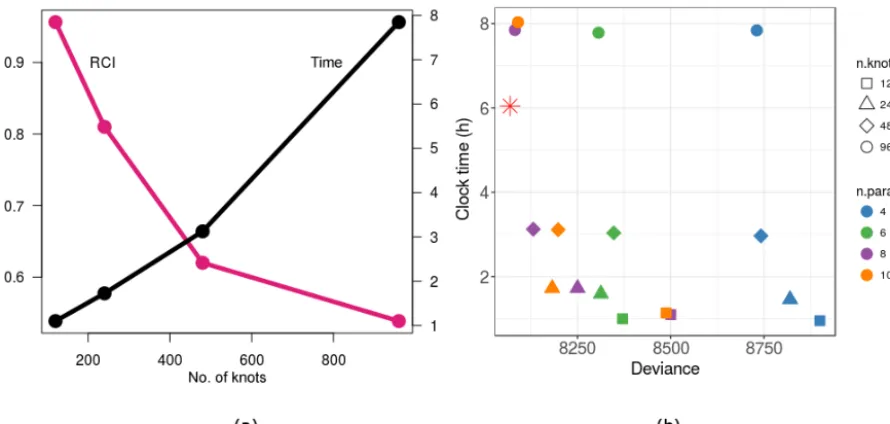
Figure 7 shows how the emulator method scales with more knots using the mlegp R package and the trade-off between wall-clock time vs. the approximation error. As expected, the post-PDA ensemble CI approaches the brute-force post-PDA CI. In other words, the RCI asymptotically converges to zero, while the clock time tends to increase with the number of knots (Fig. 7a).

The trade-off between improved model–data agreement (lower deviance values) vs. wall-clock time suggests the more we explore the parameter space (more knots), the lower the deviance becomes in general (Fig. 7b). Deviance also lowers with number of parameters targeted in general. How-ever, the best fit was not always to the model with the most parameters, and the number of parameters of the best fit var-ied with the number of knots. With a lower number of knots, fewer parameters were well constrained, but with too few pa-rameters we traded off the ability to obtain a good fit. The clock time is largely determined by the number of knots, with much lower sensitivity to the number of parameters as num-ber of knots was much greater than () the number of pa-rameters in this study.

4 Discussion

4.1 Adaptive sampling design

Our experiment against synthetic data showed that the GP model emulator method was able to recapture the true values successfully. While the posteriors of the emulators with few knots (initial round) could be wide, additional rounds of em-ulator refinement were able to constrain the posteriors better. Our test in which we proposed the cumulative number of de-sign points all at once showed that, even though we proposed the same number of knots in the end, where you propose those points in the parameter space is important, and itera-tively refining the search is a more efficient way of exploring the parameter space. This is because the initial proposal of parameters with LHC had no way of knowing which parts of parameter space are most important to explore, and thus the tails of the distributions end up oversampled and the core un-dersampled. Furthermore, without multiple iterations the co-variances among parameters are also underconstrained, un-less informative prior distributions are chosen or previously known covariances are provided. Sampling new knots from the posteriors of the previous iteration informs the algorithm about the posterior means and covariances and allows the GP to be refined adaptively. The efficiency of this workflow

could potentially be increased further by other adaptive sam-pling designs, and this remains an important area for further research. For example, Oakley and Youngman (2017) used an initial set of simulator runs to screen out low-likelihood regions to reduce the parameter space before the calibration. For a review of adaptive sampling methods, and emulator design methodologies in general, see Forrester and Keane (2009).

4.2 Emulator construction

In this study, we focused on calibrating process-based mech-anistic simulators (ecosystem models) using computation-ally cheaper emulators. Variations in emulator approach are many and can be found in Jandarov et al. (2014), Aslanyan et al. (2015), Huang et al. (2016), Oakley and Youngman (2017), and the references therein. Here we adopted the ver-sion that emulates the likelihood surface with a GP, similar to previous studies including applications with a cosmolog-ical likelihood function (Aslanyan et al., 2015), a stochas-tic natural history model (Oakley and Youngman, 2017), the Hartmann function and a hydrologic model (Wang et al., 2014), and two land surface models (Li et al., 2018). Our scheme resembles the adaptive surrogate modeling-based op-timization (ASMO) approach (Wang et al., 2014; Li et al., 2018) in terms of both the nature of the problem (calibration of a process-based mechanistic simulator) and the general scheme of the calibration algorithm. However, aside from differences in initial sampling designs and error character-izations in these studies, there are two main differences of our scheme from ASMO.

First, we run full MCMC in between the adaptive sampling steps, and on the final response surface, instead of optimiza-tion search. Hence, we were able to provide full posterior probability density distribution of the parameters targeted for calibration instead of point estimates of optimum values as in Li et al. (2018). The ASMO scheme has also been recently updated for distribution estimation using full MCMC runs (ASMO-PODE) and has been tested with the Common Land Model (Gong and Duan, 2017). An important update in our study was that we used the error estimation (variance) pro-vided by the GP model instead of only using the mean es-timates as Gong and Duan (2017) did, which allowed us to fully propagate the uncertainties to the post-PDA model pre-dictions. Earlier work (not shown) illustrated that failing to propagate the emulator uncertainty (step 5b) results in over-confident posteriors that can easily miss the true parameter in simulated data experiments.

(14)

[image:14.612.80.525.70.282.2]

Figure 7.Results of the scaling experiment.(a)Trade-off between wall-clock time and the approximation error (relative confidence interval, RCI) with increasing emulator knots.(b)The trade-off between improved model–data agreement and wall-clock time. The red star is the emulator design followed in this study for SIPNET with eight model parameters and 729 knots. Underlying data for(b)can be found in Table A9.

that are not part of the process model but are part of the sta-tistical data model (the likelihood) as well. In this study, we tested the sufficient statistics emulation for the SoilResp data and updated Gaussian likelihood precision parameter in the MCMC together with other process model parameters. This residual parameter includes both data error and model struc-tural error, and it is not possible to distinguish one from the other with this approach (van Oijen, 2017). However, when we apply the same calibration scheme to different process models at the same site, because the observation error in the data is the same, the difference in the posteriors of this residual parameter (Fig. A7) could give us clues about the model structural errors of models relative to each other, as we demonstrate in this study as a proof of concept. However, in our study, use of multiplicative bias parameter further ob-scures the difference between observation and model struc-tural error.

Indeed, implementation of a more formal way of account-ing for model structural error (also called the discrepancy be-tween model output and reality) in our emulator scheme is one of our planned next steps. Explicitly specifying a model discrepancy term and estimating it through MCMC would allow us to account for all sources of model predictive uncer-tainty (van Oijen, 2017). However, determining the expected form of discrepancy in order to learn about model param-eters realistically could be difficult due to lack of mecha-nistic knowledge of the underlying processes (Brynjarsdót-tir and O’Hagan, 2014). In that sense, accounting for dis-crepancy in model calibration is not an issue specific to em-ulator approach. For a novel approach investigating model

structural uncertainty through a modular modeling frame-work, see Walker et al. (2018), which could be useful for modeling prior knowledge about discrepancy in ecosystem models in the future. Because of the unknowns about the discrepancy functions, it is common to use GPs to model the discrepancy (Kennedy and O’Hagan, 2001). Even then, only with realistic prior constraints about the process, would calibrated model predictions be unbiased (Brynjarsdóttir and O’Hagan, 2014). For an example of addressing discrepancy in calibration that combines the likelihood-emulation ap-proach with importance sampling, see Oakley and Young-man (2017), who inflated simulator uncertainty to account for simulator discrepancy instead of explicitly specifying a prior for it in order to make the likelihood tractable. When likelihood function becomes intractable or a sufficient statis-tic does not exist, techniques using likelihood-free inference (Gutmann and Corander, 2016) or computing approximately sufficient statistics could also be a remedy (Joyce and Mar-joram, 2008).

Finally, the scheme used in this study is also compatible with various adaptive sampling designs (other than LHC), emulator models (other than GP), and MCMC algorithms (other than adaptive Metropolis–Hastings) like the ASMO-PODE scheme (Gong and Duan, 2017).

4.3 Brute force vs. emulator

(15)

finely than the emulator as expected due to the numerical approximation error in the emulator. Therefore, when com-putational time allows, brute-force methods will result in more precise posteriors and are preferred over the emulator method. However, when the model run time or the volume of data to be assimilated does not allow running long MCMC iterations, it is possible to constrain parameters in orders of magnitude less time, with far fewer model evaluations, and with much greater parallelization using the emulator method. This speedup puts model calibration within reach for large, computationally challenging models that are currently under-constrained.

In addition to just fitting the model, emulators make it practical to implement different hypotheses within a model, recalibrate the model, and test them against data repeatedly. Furthermore, emulators make it possible to calibrate com-plex models hierarchically, which would not be computation-ally feasible otherwise as hierarchical Bayesian modeling in-volves calibrating models many times at multiple spatial– temporal–experimental settings. For example, it is a known issue that site-level calibrations are not easily transferable to new sites or to larger scales (Post et al., 2017). In that sense, hierarchical Bayesian approach is an important improvement over classical Bayesian model calibrations because it for-mally accounts for the spatial and temporal variability in ecosystems and provides a structure that will help us bet-ter understand the uncertainties involved at different levels of our study systems (Clark, 2005; Thomas et al., 2017). 4.4 Autocorrelation correction and multiple data

constraints

A lack of independence in observation errors causes over-fitting of the model parameters and underestimation of pre-diction uncertainties (Ricciuto et al., 2008). It is not uncom-mon for calibration against one dataset that is given a high weight (e.g., many more observations) to cause other model outputs to perform worse. Indeed, in our calibration study, model–data agreement for NEE improved, while it was re-duced for the SoilResp variable after the brute-force cali-bration. The most common approaches to this problem in-volve arbitrary weights or ad hoc solutions to rebalance the influence of data. We addressed this issue with a novel ap-proach of explicitly modeling autocorrelation, which pro-vides a more objective and statistically rigorous approach to balancing the weights of different data. Although the NEE and LE data still influenced the calibration more than the SoilResp data, assimilating multiple data streams and bal-ancing their influence was important. For example, NEE is a result of both primary production and respiration processes, and the model outputs were sensitive to parameters involved in both of these processes. If we were to assimilate only NEE, estimated parameters contributing to NEE might have com-pensating errors (Post et al., 2017). However, including an additional constraint on model parameters contributing to

ei-ther primary production or respiration could help us distin-guish such compensation effects. Altogether, overfitting of models is a common problem in Bayesian calibration, and both the autocorrelation correction and the use of the emula-tor method practically proved to be helpful strategies. Lastly, the effect of number of assimilated data streams on emulator performance is not explicitly tested in this study; however, calibration performance of the emulator should still be pro-portional to brute force with more or fewer data streams. For studies that inspect the effect of assimilating multiple data streams on model calibration performance, see Keenan et al. (2013) and MacBean et al. (2017).

4.5 Scaling factors

In the calibration of ED2, instead of constraining the PFT parameters directly, we targeted scaling factors (SFs) for parameters that are common among PFTs, which reduces the dimensionality considerably (i.e., instead of targeting Nparameters×MPFTs, we only targetNparameters). This experi-ment showed that the emulator method with SFs could con-strain ED2 PFT parameters and improve model predictions. However, this approach assumes that therelativedifferences among PFTs are approximately correct, but that overall pro-cesses may be miscalibrated, and thus that the more likely pa-rameter space for different PFTs will be in similar regions of their prior distributions. For example, if a density-dependent mortality parameter is being targeted, the prior distributions for an early and a late successional type can be defined to rep-resent their differentiation so that the posteriors would still be different when using the SF. In our study, PDA priors for each PFT were informed by meta-analysis, therefore accom-modating for such differences amongst PFTs. By contrast, the SF approach by itself cannot, for example, converge on values in the first quartile for a certain parameter space for one PFT and in the third quartile for another PFT. We note that the SF approach is not specific to the emulator method and could also be used with brute-force algorithms to reduce dimensionality.

4.6 Approximation error vs. clock time

(16)

pa-5816 I. Fer et al.: Linking big models to big data

rameters to be constrained increases. Our scaling experiment indicates that RCI decays quickly and starts leveling off as the number of knots increases. In other words, one can stop increasing the number of knots at a stage at which the gain in terms of approximation error reduction being heavily traded off with clock time is reached. Detecting such thresholds is feasible in practice if the emulator is refined iteratively.

A similar threshold was also apparent for overall model calibration ability. While the gain, if any, in model im-provement in terms of deviance was minimal from 480 to 960 knots, the clock time required was more than doubled in our scaling experiment. This experiment also suggested that the number of model parameters we chose to constrain was an adequate choice for our setting. Targeting a few additional model parameters did not result in substantial differences in terms of overall deviance, which was expected as the targeted parameters were chosen according to their contribution to the overall model uncertainty. Thus we are confronted with the fundamental trade-off in which increasing the number of rameters requires proposing more knots to explore the pa-rameter space, which increases run time, and at some point these additional parameters provide diminishing returns. Un-derstanding this trade-off is greatly facilitated by performing an uncertainty analysis before calibration, which allows pa-rameters to be added to the calibration in order of their con-tribution to model uncertainty. Finally, we note that the shape of the clock time vs. deviance trade-off curves will vary by model as they varied by number of model parameters.

To fit the GP models in this study, we used the mlegp R package, which was found to be performing well with its de-fault settings (Erickson et al., 2018). The comparison by Er-ickson et al. (2018) shows that there are faster (such as laGP) and computationally more stable (such as GPfit) R packages available. However, laGP performs worse than mlegp unless thousands of design points are provided, and GPfit is substan-tially slower than mlegp as it is solely written in R whereas mlegp is pre-compiled in C. Finally, other packages from other platforms (such as the GPy and scikit-learn modules of Python) could outperform mlegp (Erickson et al., 2018); however, as PEcAn is mainly written in R, mlegp was an ad-equate choice for our workflow. Overall, the approximation error vs. clock-time trade-off is not independent of the soft-ware/code used to fit the GP model.

In this study, we tested emulator calibration with num-ber of parameters that are comparable to, if not higher than, previous studies with biosphere models (Ray et al., 2015; Huang et al., 2016; Gong and Duan, 2017). However, run-ning the emulator can also become infeasible. For example, with the current scheme calibrating 100 parameters would not be possible with 1003knots, asO(N3)floating point op-erations needed for the Cholesky decomposition in GP would exceed memory and wall-clock time capacities. That said, the p3 scheme is just the rule of thumb that we employed in these experiments and not an inherent limit of the emula-tor approach itself. The calibration of 100 parameters might

be possible with a much smaller number of knots (106) depending on the model. Using a sample size of about 10 times (n=10 d) the input dimension is a common recom-mendation in computer experiments with GP (Loeppky et al., 2009). But this is considered to be too small for most of the cases and using 20 times (n=20 d) larger sample sizes is suggested instead (Erickson et al., 2018). Indeed, our scaling experiment also suggests calibrating the model with fewer knots (< p3) would be possible. In practice, we would ad-vocate for performing an uncertainty analysis to reduce the dimensionality of the problem. In addition, the data would need to be strong enough to actually constrain such a large number of parameters. Still, when dimensionality becomes too large, alternative emulators could be explored, such as the nearest-neighbor GP model (which takes advantage of the fact that the nearest neighbors contribute the most informa-tion while fitting the GP model and could help reduce com-putational costs substantially for bigger datasets and a much larger number of parameters; Datta et al., 2016).

5 Conclusions

Here we introduced a framework that addresses both the computational and statistical challenges of Bayesian model calibration. We introduced a number of novel approaches, such as building an emulator on the sufficient statistics sur-face, implementing an autocorrelation correction on the la-tent time series estimated through a state-space model, and introducing a scaling factor to reduce dimensionality across PFTs. We also standardized and generalized this framework in an open source ecological informatics toolbox, PEcAn, for repeatability and use with other ecosystem models.

Our study furthers efforts toward reducing model uncer-tainties showing that the emulator method makes it possi-ble to efficiently calibrate complex models. Here we demon-strated examples and evaluated performances with terrestrial ecosystem models but the application can be generalized to any “big model”. Overall, this efficient data assimilation method allows us to conduct more calibration experiments in relatively shorter times, enabling the constraint of numerous models using the expanding number and types of data.

(17)

Appendix A A1 Study site

Bartlett Experimental Forest (44◦170N, 71◦030W) is a US Forest Service research forest located outside of Bartlett, NH, in the White Mountains (Lee et al., 2018). Species compo-sition is typical of northern hardwood forests and consists predominantly ofAcer rubrum(red maple),Fagus grandifo-lia (American beech),Betula papyrifera(paper birch), and Tsuga canadensis (eastern hemlock). Climate is also typi-cal of central New England with short summers (20◦_{C) and} long cold winters (−8◦_{C). The site is generally moist,} re-ceiving approximately 1300 mm yr−1of precipitation. Soils are sandy loam Spodosols and can become saturated during spring snowmelt.

An eddy-covariance tower (26.5 m) was installed in November 2003 at a lowland site (272 m) within the experi-mental forest. Topography near the eddy-covariance tower is flat to gently sloping but larger hills (1–3 km distant) sur-round the site. Canopy height is 19 m with a mean stand age of approximately 100 years. The eddy-covariance sys-tem consists of a LI-6262 CO2/H2O infrared gas analyzer (LI-COR, Lincoln, NE) and SAT-211/3 K three-axis sonic anemometer (Applied Technologies, Longmont, Colorado). Measurements were made at 5 Hz and fluxes were estimated every 30 min. The meteorological data used in this anal-ysis were derived from measurements made at the eddy-covariance tower for the years 2005–2006. These include air temperature above the canopy (22.3 m), soil temperature, rel-ative humidity, precipitation, above-canopy PAR, and wind speed.

The Bartlett tower footprint contains 12 vegetation inven-tory plots that follow the Forest Inveninven-tory and Analysis (FIA) design consisting of four circular 10 m radius subplots: one central and three evenly spaced at a radius of 36.5 m. Vegeta-tion plots were established in May 2004 and used to initial-ize ED2. Bradford et al. (2010) provided soil carbon and live aboveground biomass estimates for Bartlett, which we used to initialize SIPNET.

Soil respiration measurements were made manually in each plot (n=12) at permanently installed rings that are 10 cm in diameter using a soil CO2 flux chamber (LI-COR 6400-9). Soil temperature and moisture were measured con-currently using a soil temperature probe and a TDR probe. During 2006, soil respiration censuses were made approxi-mately every 4–5 days from day 138 to day 325 for a total of 39 chamber censuses.

A2 SIPNET model

The Simplified Photosynthesis and Evapotranspiration model (SIPNET) is a simple ecosystem model that can be used to interpret carbon water exchange between vegetation and the atmosphere. SIPNET has been developed from the

PnET family of models to facilitate model comparisons to flux towers (Braswell et al., 2005; Sacks et al., 2006). SIP-NET runs at a half-hourly time step. It represents relatively few processes (has two vegetation carbon pools, a single ag-gregated soil carbon pool, and a simple soil moisture sub-model), making it easier to evaluate which data contribute how much to the parameterization of each process. As a re-sult of this setup, SIPNET is a fast model (∼5.5 s per MCMC iteration in PEcAn including model execution and writing and reading model outputs), which makes it suitable for ap-plication of brute-force methods.

Forest inventory data collected in the tower footprint were used to set initial conditions in SIPNET. We fitted Bayesian models using the allometric equations available in the literature (Jenkins et al., 2004) to estimate the above-ground biomass at Bartlett through PEcAn’s allometry mod-ule. These values were in agreement with live aboveground biomass estimates by Bradford et al. (2010) whose soil car-bon pool estimates were also used to set the initial values in our SIPNET runs (Table A1).

A3 Ecosystem Demography Model

(18)

[image:18.612.74.523.81.549.2]

Figure A1.Unsmoothed, half-hourly time series comparison for NEE and LE predictions, before and after calibration.

Table A1.Initial state values used for SIPNET runs.

Pool Value Units

Above- and belowground woody biomass 9600 g C m−2ground area Initial leaf area 0 m2leaves m−2ground area

Litter biomass 200 g C m−2ground area

[image:18.612.140.449.632.702.2]

(19)

[image:19.612.126.468.101.215.2]

Table A2.The prior and posterior distributions of the constrained SIPNET parameters.

Parameter Prior Posterior (emulator) Posterior (brute force)

[image:19.612.91.507.279.483.2]

SOM respiration rate unif(0.001, 0.3) weibull(1.62, 0.13) norm(0.1, 0.009) Soil respirationQ10 unif(1.4, 3.0) lnorm(0.697, 0.24) lnorm(0.39, 0.046) Soil WHC unif(0.1, 36.0) lnorm(2.95, 0.31) lnorm(2.7, 0.035) Half saturation PAR unif(4.0, 27.0) weibull(3.74, 17.5) lnorm(2.8, 4.5×10−2) dVPDSlope unif(0.01, 0.25) weibull(2.26, 7e-02) norm(0.08, 2.6×10−3) Seasonal leaf growth unif(0.0, 252.0) norm(150.6, 46.8) norm(145, 10.8) psnTOpt unif(5.0, 40.0) norm(12.07, 35.7) weibull(336, 39.9) Leaf turnover rate unif(0.03, 6.0) norm(5.14, 1.9) lnorm(1.64, 5×10−2)

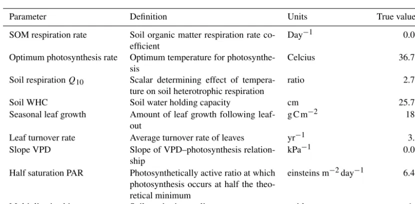
Table A3.Calibrated SIPNET parameters and the “true” values used to produce the synthetic data.

Parameter Definition Units True values

SOM respiration rate Soil organic matter respiration rate co-efficient

Day−1 0.01

Optimum photosynthesis rate Optimum temperature for photosynthe-sis

Celcius 36.75

Soil respirationQ10 Scalar determining effect of tempera-ture on soil heterotrophic respiration

ratio 2.75

Soil WHC Soil water holding capacity cm 25.75

Seasonal leaf growth Amount of leaf growth following leaf-out

g C m−2 180

Leaf turnover rate Average turnover rate of leaves yr−1 3.2

Slope VPD Slope of VPD–photosynthesis relation-ship

kPa−1 0.05

Half saturation PAR Photosynthetically active ratio at which photosynthesis occurs at half the theo-retical minimum

einsteins m−2day−1 6.46

Multiplicative bias Soil respiration scaling constant unitless 1.5

Table A4.Calibrated ED2 parameters.

Parameter Definition Units

Stomatal slope Slope of relation between stomatal conductance andA ratio Quantum efficiency Efficiency with which light is converted into fixed carbon fraction

Vcmax Maximum rubisco carboxylation capacity µmol CO2m−2s−1

Cuticular conductance Leaf (cuticular) conductance when stomata fully closed µmol H2O m−2s−1 Growth respiration factor Proportion of daily carbon gain lost to growth respiration fraction

Fine root allocation Ratio of fine root to leaf biomass ratio r_stsc Fraction of structural pool decomposition going to

het-erotrophic respiration

fraction

Decay rate stsc Intrinsic decay rate of structural pool soil carbon 1/day Resp. temperature increase Determines how rapidly heterotrophic respiration increases

with increasing temperature

1/K

[image:19.612.81.512.545.703.2]

(20)

[image:20.612.46.549.155.306.2]

Table A5.The PDA prior (meta-analysis posterior) approximated parametric distributions of the targeted ED2 parameters.

Plant functional type physiological parameters

t.EH t.LC t.LH t.NMH t.NP

Stomatal slope gamma(19.7, 2.97) weibull(2, 10) weibull(2, 10) weibull(2, 10) weibull(2, 10)

Quantum efficiency gamma(16.6, 279) norm(0.08, 0.014) weibull(2.9, 0.07) lnorm(-3.28, 0.08) gamma(82, 1.4×103)

Vcmax norm(74.9, 9.8) weibull(1.7, 80) norm(60.5, 11.9) gamma(37.8, 0.53) weibull(2.2, 80)

Cuticular conductance lnorm(9.4, 0.7) lnorm(9.4, 0.7) lnorm(9.4, 0.7) norm(9988, 497) lnorm(9.4, 0.7)

Growth respiration factor beta(4.06, 7.2) beta(2.63, 6.52) beta(4.06, 7.2) beta(2.63, 6.52) beta(2.63, 6.52) Fine root allocation gamma(16.59, 23.32) lnorm(−0.25, 1) gamma(9.13, 8.22) gamma(9.44, 8.82) lnorm(−0.25, 1)

Soil biogeochemistry (decomposition) parameters

r_stsc beta(1, 1)

Decay rate stsc unif(0.005, 0.75)

Resp. temperature increase unif(0.05, 0.2)

t.EH: temperate early hardwood; t.LC: temperate late conifer; t.LH: temperate late hardwood; t.NMH: temperate north mid-hardwood; t.NP: temperate northern pine.

Table A6.The emulator PDA approximated parametric posterior distributions of the targeted ED2 parameters.

Plant functional type physiological parameters

t.EH t.LC t.LH t.NMH t.NP

stomatal slope lnorm(1.48, 0.13) gamma(4.01, 1.6) gamma(4.01, 1.6) gamma(4.01, 1.6) gamma(4.01, 1.6)

quantum efficiency lnorm(−2.8, 0.11) norm(0.08, 6.3×10−3) gamma(35.8, 541) lnorm(−3.3, 0.04) lnorm(−2.8, 0.05)

Vcmax norm(47.3, 3.45) gamma(2.83, 1.04) norm(27.1, 4.17) norm(42.9, 2.85) weibull(2.4, 6.4)

cuticular conductance norm(9.85, 0.385) norm(9.85, 0.385) norm(9.85, 0.385) norm(10 308, 273) norm(9.85, 0.385) growth respiration factor beta(3.59, 7.47) beta(2.29, 6.8) beta(3.59, 7.47) beta(2.29, 6.8) beta(2.29, 6.8) fine root allocation gamma(30.7, 7.47) lnorm(−0.3, 0.73) gamma(16.7, 15.6) gamma(17.3, 16.8) lnorm(−0.3, 0.73)

Soil biogeochemistry (decomposition) parameters

r_stsc beta(1, 1.98)

decay rate stsc lnorm(−2.97, 1.02)

resp. temperature increase lnorm(−2.16, 0.28)

[image:20.612.47.552.486.639.2]

(21)

[image:21.612.118.481.236.513.2]

(22)

[image:22.612.52.548.156.599.2]

(23)

[image:23.612.52.546.157.604.2]

(24)

[image:24.612.101.497.74.387.2]

Figure A5.ED2 decomposition and scaling factor posterior density distributions. Parameters common to all ED2 PFTs ending with the suffix “SF” were targeted through the scaling factor.

[image:24.612.128.468.445.677.2]

(25)

[image:25.612.309.547.315.531.2]

Table A7.Links to the workflow IDs. The input–output files as-sociated with each workflow can be accessed via the history ta-ble at the following link http://pecan2.bu.edu/pecan/history.php, last access: 30 September 2018. Or each workflow can be accessed directly by replacing the workflow ID at the end of the follow-ing link: http://pecan2.bu.edu/pecan/08-finished.php?workflowid= 1000008379, last access: 30 September 2018. The left frame on the page can be used to navigate through PEcAn settings and input and output files. If you wish to conduct further vi-sualizations or analysis on the MCMC samples, you can first select the “mcmc.list.pda***.Rdata” file (*** being the ensem-ble IDs given by the workflow) under the “PEcAn Files” drop-down menu on the left frame. By clicking “Show File” button you can download the raw MCMC outputs to your own ma-chines. If you would like to display posterior density distributions, first select either soil or plant physiology under the “PFTs/PFT” menu on the left frame. Next, under the “PFTs/Output” drop-down menu, select “posteriors.pda.***.pdf” and click “Show PFT Output”. The red line would be the posterior density plot and the black line would be the approximated parametric distribu-tions (such as the ones reported in Tables A2 and A6) fitted by PEcAn’s approx.posterior function that can be found under pecan/modules/meta.analysis/R/approx.posterior.R.

Model Experiment Workflow ID

SIPNET Pre-PDA EA/UA 1000008379

SIPNET Emulator PDA – synthetic data 1000009295

SIPNET Emulator PDA – real data 1000009249

SIPNET Emulator post-PDA EA 1000009309

SIPNET Brute-force PDA – real data (chain 1) 1000008530 SIPNET Brute-force PDA – real data (chain 2) 1000008531 SIPNET Brute-force PDA – real data (chain 3) 1000008532

SIPNET Brute-force post-PDA EA 1000008923

ED2 Pre-PDA EA/UA 1000009051

ED2 Emulator PDA – real data 1000009052

ED2 Emulator post-PDA EA 1000009052

[image:25.612.48.285.334.471.2]

PDA: parameter data assimilation; EA: ensemble analysis; UA: uncertainty analysis.

[image:25.612.51.283.519.668.2]

Figure A7. Posterior probability density distribution of variance (reciprocal of the precision, 1/τ) parameter of the soil respiration likelihood after emulator PDA.

Table A8. Links to the workflow IDs of scaling experi-ments. Parameters targeted are in this order cumulatively: som_respiration_rate, soil_respiration_Q10, soilWHC, psnTOpt (4), leafGrowth, leaf_turnover_rate (6), half_saturation_PAR, dVPDSlope (8), AmaxFrac, dVpdExp (10).

Model No. of parameters No. of knots Workflow ID

SIPNET 4

960 1000009310 480 1000009311 240 1000009312 120 1000009313

SIPNET 6

960 1000009314 480 1000009315 240 1000009316 120 1000009317

SIPNET 8

960 1000009318 480 1000009319 240 1000009320 120 1000009321

SIPNET 10

(26)

[image:26.612.96.504.282.517.2]

Table A9.Scaling experiment results showing the trade-off between wall-clock time and the approximation error with increasing emulator knots.

m n Model run time (s) GP fitting (s) 100 K MCMC (s) Deviance