Nonlinear Identication of the Position Sled Dynamics of a
CD Player
Jonas Sjöberg
Dept. of Signals and System Chalmers University of Technology
Gothenburg, Sweden.
Per-Olof Gutman
yFaculty of Agricultural Eng. Technion - Israel Inst. of Technology
Haifa 32000, Israel.
Abstract
This contribution concerns the identification of the dynamics of a sled carrying the op-tics housing of a CD player. The memory access time of the CD player depends, among other factors, on the settling time of the sled after a step change. This contribution focusses on the oscillations at the end of a step response. Measured closed-loop data are used to identify different types of black-box models of the sled dynamic. First linear models are concerned, and then different types of nonlinear models. The different types of models are compared and discussed. Due to poor excitation of the plant, some conclusions are uncer-tain. However, it is clear that the nonlinear models give better simulation performance on validation data than the linear ones. Also, the oscillations at the end of a step response seem to be controller induced. Therefore, it seems appropriate to use different models, and then also different controllers, at different parts of a step response.
1 Introduction
The speed of a CD player can be measured in different ways. Often, only the rotational speed of the disc is used as a measure. This is a relevant measure in a steady state reading situation, i.e., when the CD player is following a certain track on the disc. As described in Section 2 the CD player concerned in this paper uses multiple beams to increase the steady state reading speed without increasing the rotation speed the disc.
Another important measure of speed is the memory access time. It is defined as the time it takes to position the laser beam at a given track and to start reading there. To obtain a short memory access time the step response of the optics housing has to be fast and the settling time at the end of the step response must be short. It is first when the oscillations at the end of the step response are less than some threshold value that data retrieval can start.
In this work we concentrate on this settling time at the end of a step response and the dynamics of the sled, carrying the the optics housing, is identified in this region.
There are several aggravating factors which makes the identification hard. First, the resolu-tion of the output signal, the posiresolu-tion of the sled, is limited by fairly large quantizaresolu-tion errors. This means that only a crude measure of the output is available. Second, the system is operat-ing in closed loop, and at the end of a step in the reference signal, there is no external excitation
Email: [email protected]. Financial support from Lady Davis Foundation, Jerusalem, Israel and the Swedish Research Council for Engineering Science (TFR) is gratefully acknowledged.
y
of the system. The only excitation on the system is the measurement noise on the output. As we will see, these in-sufficiences in the data, to some extent, limits the possible faith in the obtained models.
The identification procedure follows the general principle “Try Simple Things First”, and, therefore, starts with linear black-box models. Standard algorithms are used, as described in, e.g., (Ljung, 1999; Söderström and Stoica, 1989). See also some more introductory books on identification, e.g., (Johansson, 1993; Ljung and Glad, 1994).
A main problem when nonlinear black-box models are considered, is that there are so many different possibilities of model structures. Here, we will follow a strategy where an obtained linear model is used as starting point for the nonlinear system identification. This makes it possible to initialize nonlinear models with reasonable good parameter values, as described in (Sjöberg and Ngia, 1998) or in (Sjöberg, 1997).
Other interesting approaches to nonlinear system identification are described in (Murray-Smith and T.A., 1997). Some possible nonlinear model structures can be found in (Billings
et al., 1992), and in the references therein. The paper (Sjöberg et al., 1995) discusses the general
problems with nonlinear identification, and techniques how the problems can be handled. The paper is organized as follows. In Section 2 the system is described, and Section 3 defines the identification problem. Linear models are considered in Section 4 and nonlinear models in Section 5. The paper is concluded in Section 6.
2 The plant
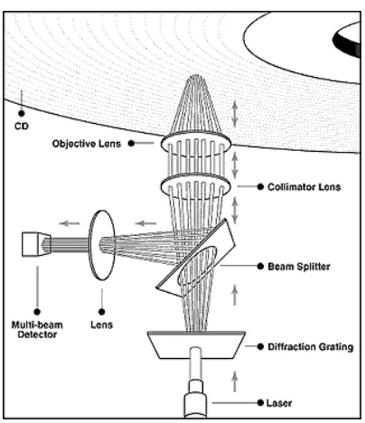
The multiple beam CD player, depicted in Figure 1, is developed by Zen Research Ltd1. The multiple beam approach to illuminating and detecting multiple tracks uses a diffracted laser beam in conjunction with a multiple beam detector array. A conventional laser diode is sent through a diffraction grating which splits the beam into seven discrete beams, spaced evenly to illuminate seven tracks. The seven beams pass through a beam splitting mirror to the objective lens and onto the surface of the disc. Focus and tracking are accomplished with the central beam. Three beams on either side of the center are readable by a detector array as long as the center is on track and in focus.
The reflected beams return via the same path and are directed to the multiple beam detector array by the beam splitter mirror. The detector contains seven discrete detectors spaced to align with seven reflected tracks. Conventional detectors are also provided for focus and tracking.
The control design uses a conventional approach to tracking and seeks. In particular, the fine positioning of the optics is controlled in an inner loop, whereas the optics housing resides on a sled with which the course positioning is done. In this paper we will identify the sled po-sitioning dynamics from measured signals from a closed loop experiment on an experimental laboratory set-up that does not necessarily reflect neither the performance nor the sled dynam-ics of production CD-players.
Performance is far greater than that of conventional drives because the multi-beam technol-ogy allows for lower, more disc tolerant rotational speeds.
1
Figure 1: Illustration of the multiple beam CD player.
3 The Data
The closed loop system is depicted in Figure 2. The output signal, y(t)is the position of the
sled (in meters), and the input,u(t)is the applied voltage (in Volts) to the servo acting on the
sled. The sampling interval of the signals isT s
=0:455ms.
Contr.
y r
u
v
Plant
Figure 2: System description.
Data from a step response experiment is shown in Figure 3. The reference signal is a low-pass filtered step (not shown in the plot) and the output signal follows close to the reference signal until the step amplitude is reached. At the end of the step response the output oscillates around the reference value. This is barely seen in the Figure 3. >From a control perspective, it is interesting to understand the plant dynamics at a new, constant, reference value. With such knowledge the control may be improved so that the settling time can be shortened. Therefore, we focus the identification on the end of the step response and Figure 4 this part of the step response in Figure 3 is shown.
[image:3.595.173.455.472.554.2]0 50 100 150 200 250 300 350 −0.038
−0.036 −0.034 −0.032 −0.03 −0.028 −0.026 −0.024
OUTPUT #1
0 50 100 150 200 250 300 350 −1
−0.5 0 0.5 1
[image:4.595.217.410.99.263.2]INPUT #1
Figure 3: Step response data of the CD sled versus time samples. a) Plant output signal,u(t).
b) Plant input signal,y(t).
The sensor measuring the position of the sled gives quantized values. In between the quan-tization levels the output is not observable, and this fact limits the control performance when the output is near the reference signal. Consider the second data half in Figure 4. >From the
0.07 0.08 0.09 0.1 0.11 0.12 0.13 0.14 0.15
−0.0245 −0.0244 −0.0243 −0.0242 −0.0241 −0.024 −0.0239 −0.0238
Figure 4: Reference signal (solid), measured output signal (dashed), and (scaled) control signal (dotted).
figure you see that the control signal looks the same, but with opposite sign, whenever the po-sition error is one quantization step from the correct value; a short pulse in the control signal moves the sled to to the correct position. However, after the first pulse a second pulse follows which moves the sled so that an error with opposite sign is obtained. We can, therefore, con-clude that the controller is badly tuned for this signal range. From the figure it is clear that the controller induces a limit cycle.
Although these oscillations about the reference value are not wanted, they do not cause any problem in the system. The reason for this is that the oscillations are compensated in a second control loop controlling the lens on the sled.
Instead, we will focus on the first data half in Figure 4, before the oscillations are of ampli-tudeone quantization step. It is the oscillations in this data range which limits the access
[image:4.595.216.412.380.537.2]information can start. Hence, with a better model of the plant in this domain it is possible to design a better controller.
4 Linear System Identification
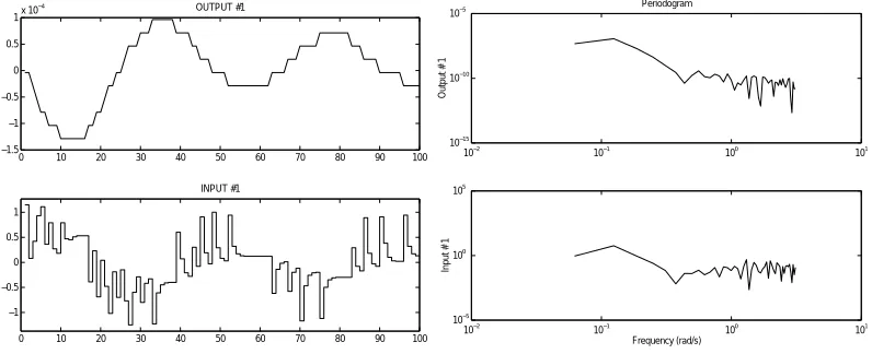
In the previous section the interesting range of the data was defined. The identification data chosen according to that description are shown in Figure 5. A second data set from a similar step response is used for validation. Both the identification and the validation data sets consist of about100samples.
0 10 20 30 40 50 60 70 80 90 100
−1.5 −1 −0.5 0 0.5
1x 10
−4 OUTPUT #1
0 10 20 30 40 50 60 70 80 90 100
−1 −0.5 0 0.5 1 INPUT #1 10−2 10−1 100 101 10−15 10−10 10−5
Output # 1
Periodogram
10−2 10−1 100 101
10−5 100
105
Frequency (rad/s)
[image:5.595.115.513.246.408.2]Input # 1
Figure 5: Identification data. a) Time-domain. b) Frequency domain.
Some trial and error shows that there is no reason to use larger than first order models. The first model structure considered is an ARX model is defined by
y(t)= B(q) A(q) u(t)+ 1 A(q) e(t) (1)
and the second model structure is an OE model defined by
y(t)=
B(q)
F(q)
u(t)+e(t) (2)
whereA(q)=1+a 1
q -1
,B(q)=b 1
q -1
,F(q)=1+f 1
q -1
, andqis the shift operator defined as
q -1
u(t)=u(t-1). The second exiting signal,e(t), is a non-measured white noise signal which
is used to explain the discrepancy between measured values and data.
The ARX and the OE differ only in the noise model. In most problems there is no reason why you should choose the noise model as 1=A(q), as for the ARX model. Instead, the ARX
The parameter estimate is defined as the minimum of the summed-squared error (SSE) using the identification data, i.e.,
V N = 1 N N X t=1
(y(t)-y(t))^
2
(3)
is minimized with respect toa 1, and
b
1, or, for the OE model, f
1, and b
1.
Nis the number of
identification data.
0 20 40 60 80 100 120
−1.5 −1 −0.5 0 0.5
1x 10
−4 Fit: 4.6261e−005
0 20 40 60 80 100 120
−1.5 −1 −0.5 0 0.5 1
1.5x 10
[image:6.595.114.511.220.388.2]−4 Fit: 1.4867e−005
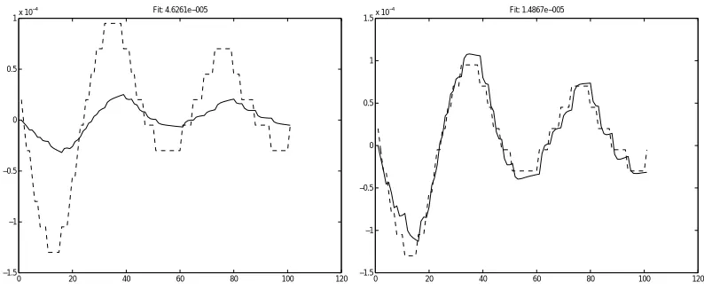
Figure 6: Simulation on validation data with a first order a) ARX model b) OE model.
In Figure 6 the simulation results for first order ARX and OE models on validation data are shown. Although, the ARX model has a good prediction performance (not shown), its simulation performance is very poor.
The good prediction ability of the ARX model can intuitively be explained by the fact that the output signal is constant except at the jumps between the quantization levels. Therefore, an ARX model consisting of a pure integration,y(t)^ =y(t-1), would give a perfect one-step
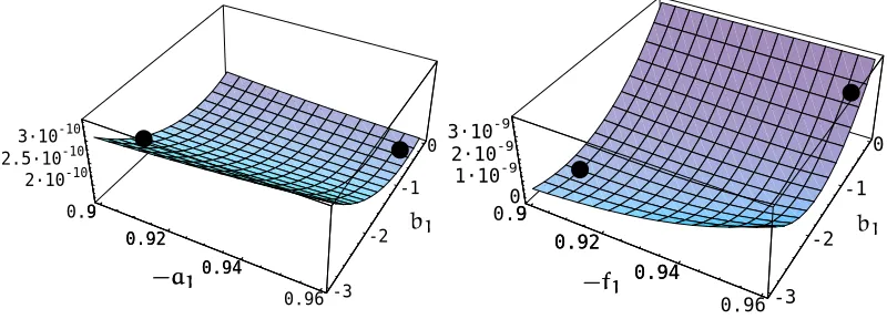
prediction except at the jumps. Indeed, in Figure 8 the SSE criteria are shown for the ARX, and the OE models as functions of the parameters, and the models’ poles are close to one.
The prediction with the OE model is based solely on the measured input signal, and it can, therefore, not exploit the locally constant output.
The failure of the ARX model can also be theoretically motivated. The expectation of the SSE criterion on new data can be expressed in the frequency domain as
¯
V ()=
1 4 Z -h jG 0 (e i!
)-G(e
i! )j 2 u (!)+ (!) i 1 jH(e i! j 2 d! (4)
whereG(q)is the plant model,G 0
(q)is the true plant, andH(q)is the noise model. u
(!)and
u
(!)are the spectra of the input signal and the noise
2. See, e.g., (Ljung, 1999).
Equation (4) shows that the model fit will be frequency weighted with the inverse of the noise model. In the ARX case this weighting becomesjA(e
i! j
2
. IfA(q)has a root near1then
the estimated model can be expected to be very poor at low frequencies. This is exactly what happens with the ARX model, and this explains the poor simulation performance.
2The noise, denoted
For the OE model this does not happen since its noise model is1, and hence constant over
the whole frequency domain.
The expected quality (4) is strictly valid only if the input,u(t), is independent on the noise,
e(t). This does not hold in our case since the data come from a closed loop experiment.
There-fore, we cannot have too much trust in (4). In Figure 7 the cross-correlation between the input signal and the residuals, i.e., the estimate ofe(t), is shown. For (4) to be strictly valid the cross
correlation should be zero.
−10 −8 −6 −4 −2 0 2 4 6 8 10
−0.4 −0.2 0 0.2 0.4
Autocorrelation of residuals for output 1
−10 −8 −6 −4 −2 0 2 4 6 8 10
−1 −0.5 0 0.5
[image:7.595.216.411.209.373.2]Samples Cross corr for input 1and output 1 resids
Figure 7: Correlation of the residuals on validation data for the first order ARX model.
From Figure 8 it is evident that the criteria have a valleys for both the ARX and the OE model. This means that the parameters can be varied along the valley without the criterion changing substantially. This verifies our earlier worries that the system is poorly excited due to the constant reference signal.
0.9 0.92
0.94
0.96 -3 -2
-1 0 2·10-10
2.5·10-10 3·10-10
.9 0.92
0.94
-a 1 -a
1
b 1
0.9
0.92
0.94
0.96-3 -2
-1 0
0 1·10-9 2·10-9 3·10-9
9
0.92
0.94
-f 1 -f
1
b 1
Figure 8: The SSE criterion versus the model parameters for the first order models a) ARX b) OE. The minima for the two models are marked with dots (in both plots). The value of the pole is on the-a
1(
-f
1axis, and both models have poles near 1.
[image:7.595.113.513.500.644.2]every second data sample. In this way the sampling time is doubled.
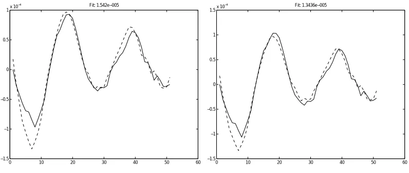
The down sampled data are shown in Figure 9. Notice that the down sampling removed the local constant feature of the output signal. The down sampling also halves the number of data so that the identification data set consists of about50samples.
Figure 10 shows simulation with OE and ARX models on down sampled data. The ARX model performs much better on the down sampled data. The reason for this is that high fre-quency noise was removed in the down sampling.
0 10 20 30 40 50 60
−2 −1 0 1
2x 10
−4
Output # 1
Input and output signals
0 10 20 30 40 50 60
−1 −0.5 0 0.5 1
Time
Input # 1
10−1
100
101
10−15 10−10
10−5
Output # 1
Periodogram
10−1
100
101
10−5
100
105
Frequency (rad/s)
[image:8.595.115.512.211.375.2]Input # 1
Figure 9: Down sampled identification data. a) Time-domain. b) Frequency domain.
0 10 20 30 40 50 60
−1.5 −1 −0.5 0 0.5
1x 10
−4 Fit: 1.542e−005
0 10 20 30 40 50 60
−1.5 −1 −0.5 0 0.5 1
1.5x 10
−4 Fit: 1.3436e−005
Figure 10: Simulation on validation data with first order a) ARX model b) an OE model.
In Figure 11 the simulation result of a second order OE model is shown. The performance is slightly better than the first order models. However, the poles are real, as shown in Figure 11 b), and this indicates that the oscillations in the output signal could be controller induced. However, due to the poor excitation of the plant this conclusion is uncertain.
5 Nonlinear System Identification
[image:8.595.115.513.431.599.2]0 10 20 30 40 50 60 −1.5
−1 −0.5 0 0.5 1
1.5x 10
−4 Fit: 1.1734e−005
−1 −0.5 0 0.5 1
−0.8 −0.6 −0.4 −0.2 0 0.2 0.4 0.6 0.8
[image:9.595.116.513.103.269.2]Poles (x) and Zeros (o)
Figure 11: Second order OE model a) simulation on validation data. b) poles () and zeros (o).
The linear models from the previous section will be used to define different nonlinear mod-els. Using a linear model for the initialization of a nonlinear model, as described in (Sjöberg and Ngia, 1998; Sjöberg, 1997), has the advantage that the performance of the initial nonlinear model is equal to that of the linear one. In this way, stability of the model can be assured and the risk to end up in a bad local minimum decreases. Starting at the initialization, the parameters of the nonlinear model are tuned by a iterative minimization algorithm, so that all parameters are fitted to the identification data.
The nonlinear models are defined by adding small nonlinear parts to the linear models. In this way the nonlinear models inherit most of their structure from the linear ones. The defined nonlinear models become “close” to being linear, and the nonlinearity is constrained to a part of the nonlinear model. By following a trial and error procedure, different possible ways to add nonlinearities to the linear models are investigated.
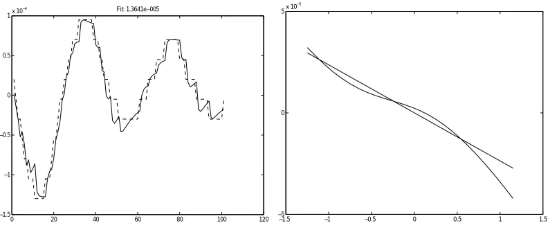
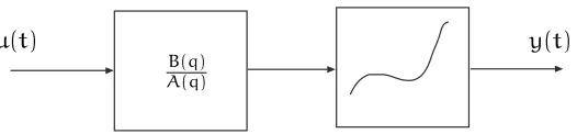
Figure 12 depicts a nonlinear OE, (NOE), model structure defined by adding a nonlinearity in parallel to the linear first order OE model, i.e., the model is described by
^
y(t)=-f
1 ^
y(t-1)+b
1
u(t-1)+g(;u(t-1)) (5)
where g(;) is a one-hidden layer feedforward neural net with 2 hidden neurons, and is
the parameter vector of the net. This model structure is equivalent to a Hammerstein model. Figure 13 depicts the simulation result using this first order NOE Hammerstein model. The
Σ
linear
^
y(t-1)
^ y(t)
[image:9.595.206.408.600.683.2]u(t-1) g(;)
Figure 12: First order NOE model with nonlinearity only on the lagged input value.
0 20 40 60 80 100 120 −1.5
−1 −0.5 0 0.5
1x 10
−4 Fit: 1.3641e−005
−1.5 −1 −0.5 0 0.5 1 1.5
−5 0
5x 10
[image:10.595.116.512.103.269.2]−5
Figure 13: First order NOE model with nonlinearity only on the lagged input value. a) Simula-tion on validaSimula-tion data. b) Estimated dependence onu(t-1)for the linear- and the nonlinear
model.
is also depicted in Figure 13 together with that for the linear OE model. The deviation from the linear model is most clear at high input amplitudes. A possible interpretation could be that the nonlinearity is caused by a saturation.
Similar simulation result to that shown in Figure 13 is also obtained if the NOE model structure (5) is changed so that it becomes nonlinear also in past output values, i.e.,
^
y(t)=-f
1 ^
y(t-1)+b
1
u(t-1)+g(^y(t-1);u(t-1)): (6)
where the nonlinear mappingg(;)is a small neural net.
>From the results so far, we can conclude that different nonlinear model structures give models superior to the linear ones. Therefore, the exact form of the nonlinear model does not seem to be crucial for the simulation result, the important feature is instead that some nonlinearity is introduced in the model.
Consider now the down sampled data. We start with a second order model. Several differ-ent types of second order NOE models have been tried and the following model structure has the best simulation performance on validation data:
^
y(t)=f
1 ^
y(t-1)+f
2 ^
y(t-2)+b
1
u(t-1)+g(u(t-1))+b
2
u(t-2) (7)
The nonlinearityg()is a one-hidden layer feedforward net with one single hidden neuron. It
takes only one of the lagged values input as argument,u(t-1). The model is illustrated in
Figure 14 a). Figure 14 b) shows the simulation result with the second order NOE model. The RMS value is13% lower than the corresponding linear model. Compare with Figure 11.
In Figure 15 the dependence onu(t-1)of the NOE model (7) is shown together with the
corresponding relationship for the linear OE model. Like all other estimated nonlinearities there are larger deviation between from the linear model at large amplitudes.
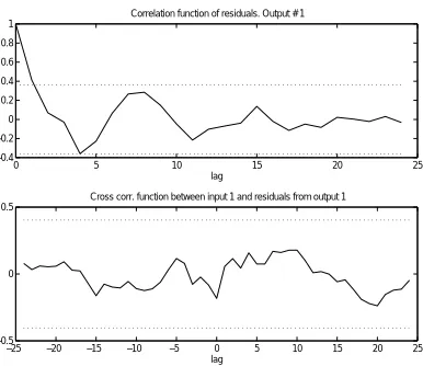
Consider now a Wiener model, a linear dynamic model followed by a static nonlinearity, as depicted in Figure 16. The linear part of the model consists of an OE model, and the nonlinear part is a feedforward net with one single neuron in parallel with a linear mapping. The model contains 6parameters. The simulation with the fitted Wiener model is shown in Figure 17 a)
Σ
linear
^
y(t-1)
^
y(t-2)
^ y(t)
u(t-1)
u(t-2)
g(;)
0 10 20 30 40 50 60
−1.5 −1 −0.5 0 0.5
1x 10
−4 Output 1, fit: 1.023e−005
[image:11.595.111.513.120.292.2]Solid: Model output, Dashed: Measured output
Figure 14: NOE 221 model with nonlinearity only on the first lagged input value. a) Illustrated model. b) Simulation on validation data.
−1 −0.8 −0.6 −0.4 −0.2 0 0.2 0.4 0.6 0.8 1
−8 −6 −4 −2 0 2 4
6x 10
[image:11.595.216.413.385.555.2]−5
Figure 15: The nonlinear relation in (7) compared to the one in the corresponding linear model.
y(t) u(t)
B(q)
A(q)
[image:11.595.173.436.636.697.2]0 10 20 30 40 50 60 −1.5
−1 −0.5 0 0.5
1x 10
−4 Output 1, fit: 9.2816e−006
Solid: Model output, Dashed: Measured output −1.50 10 20 30 40 50 60 70
−1 −0.5 0 0.5
1x 10
[image:12.595.115.512.161.330.2]−4
Figure 17: Simulation of a first order Wiener model on validation data.
0 5 10 15 20 25
−0.4 −0.2 0 0.2 0.4 0.6 0.8 1
Correlation function of residuals. Output # 1
lag
−25 −20 −15 −10 −5 0 5 10 15 20 25
−0.5 0 0.5
Cross corr. function between input 1 and residuals from output 1
lag
[image:12.595.218.411.490.657.2]between the residuals and the the inputs signal is shown. The nonlinear behavior is most predominant at large output values. There are two, possible, easy explanation for this; there might be some kind of saturation, or, since the speed becomes zero at the turning points, there might be problem with friction at these points.
6 Conclusions
The dynamics of a the position sled of a CD player at the settling after a reference step is identified.
The data are collected in closed loop, and the external excitation is poor. These aggravating circumstances make the results less reliable. The coarse quantization of the output signal also gives problems.
Several different linear and nonlinear models are investigated, and the simulation results of the well performing models are presented in the paper.
The identification procedure of the nonlinear models follows a stepwise procedure where the linear black-box models are used to define and initialize the nonlinear black-box models. By keeping the nonlinear model, and adding smaller nonlinear parts to it, more constrained nonlinear models with less parameters, are obtained.
Best simulation results on validation data is obtained with a first order Wiener model af-ter down sampling of the data with a factor 2. However, superior higher order models can
probably be identified if data exciting the system better are made available. In particular, if the main non-linearity is friction, it could be possible to assume a model structure that includes a non-linear friction feedback from the sled velocity to the force input. Such an attempt would probably also demand that the position measurement quantization is made smaller.
References
Billings, S., H. Jamaluddin, and S. Chen (1992). “Properties of neural networks with application to modelling non-linear dynamical systems,” Int. J. Control, 55, no. 1, pp. 193–224.
Johansson, R. (1993). System Modeling & Identification, Prentice-Hall, Inc., Englewood Cliffs, New Jersey 07632.
Ljung, L. (1999). System Identification: Theory for the User, Prentice-Hall, Englewood Cliffs, NJ, 2nd edn.
Ljung, L. and T. Glad (1994). Modeling of Dynamic Systems, Prentice Hall, Englewood Cliffs, N.J.
Murray-Smith, R. and J. T.A. (eds.) (1997). Multiple Model Approaches to Modelling and Control, Taylor Francis Ltd, 1 Gunpowder Square, London EC4A 3DE.
Sjöberg, J. and L. Ngia (1998). Nonlinear Modelling, Advanced Black-Box Techniques, Kluwer Aca-demic Publisher, chap. Neural Nets and Related Model Structures for Nonlinear System Identification, pp. 1–28.
Sjöberg, J., Q. Zhang, L. Ljung, A. Benveniste, B. Deylon, P.-Y. Glorennec, H. Hjalmarsson, and A. Juditsky (1995). “Non-linear black-box modeling in system identification: a unified overview,” Automatica, 31, no. 12, pp. 1691–1724.