Galley
Pro
of
Vol. 8, No. 2, (2018), pp 119–140 DOI:10.22067/ijnao.v8i2.64202
An efficient hybrid algorithm based on
genetic algorithm (GA) and
Nelder–Mead (NM) for solving
nonlinear inverse parabolic problems
H. Dana Mazraeh∗ and R. Pourgholi
Abstract
In this paper a hybrid algorithm based on genetic algorithm (GA) and Nelder–Mead (NM) simplex search method is combined with least squares method for the determination of temperature in some nonlinear inverse parabolic problems (NIPP). The performance of hybrid algorithm is estab-lished with some examples of NIPP. Results show that hybrid algorithm is better than GA and NM separately. Numerical results are obtained by im-plementation expressed algorithms on 2.20GHz clock speed CPU.
Keywords: Hybrid; NIPP; Nonlinear inverse parabolic problem; Genetic algorithm; Nelder–Mead; The least squares method.
1 Introduction
Most phenomena in real world are described through nonlinear equations, and these type of equations have attracted lots of attention among scientists. For example, consider that the sun shines in a room, and it begins to warm up. Apparently, the physical property here is the temperature, which is a function of the time and space, and the governing equations that represent the temperature variations, are a nonlinear parabolic problem (NPP) [1].
∗Corresponding author
Received 5 May 2017; revised 25 November 2017; accepted 13 June 2018 H. Dana Mazraeh
School of Mathematics and Computer Science, Damghan University, P.O.Box 36715-364, Damghan, Iran. e-mail:[email protected]
R. Pourgholi
School of Mathematics and Computer Science, Damghan University, P.O.Box 36715-364, Damghan, Iran. e-mail:[email protected]
Galley
Pro
of
In linear and nonlinear parabolic problems, we are usually facing a prob-lem, where problem conditions, initial conditions, and boundary conditions are identified and in the main equation only the equation main function is unknown. In fact, there is just one unknown factor at the problem. These problems are called direct problems.On the contrary there is another category of problems. In this category, in addition to the main equation of the problem, there are another unknown parts such as boundary conditions. This type of problems are called inverse problems [12].
In the present paper, we consider nonlinear inverse parabolic problems as the following form:
Ut=ϕ(x, t, U, Ux, Uxx), (x, t)∈(0,1)×(0, tm), (1a) with the initial condition
U(x,0) =f(x), x∈[0,1], (1b) and the boundary conditions
U(0, t) =p(t), t∈[0, tm], (1c)
U(1, t) =q(t), t∈[0, tm], (1d) and the overspecified condition
U(α, t) =s(t), t∈[0, tm], 0< α <1, (1e) where ϕis some nonlinear expression in terms of U, Ux,Uxx, andf(x) is a continuous known function. p(t) andq(t) are infinitely differentiable known functions, andtM represents the final existence time for the time evolution of the problem, while functionq(t) is unknown, which remains to be determined from some interior temperature measurements (overspecified condition).
Galley
Pro
of
space. It is successfully applied to nonlinear optimization problems for which derivatives may not be known. However, the Nelder–Mead technique is a heuristic search method that can converge to nonstationary points [16] on problems that can be solved by alternative methods.Our main purpose is to find an unknown boundary condition in NIPPs using our proposed hybrid method. Because by having this unknown bound-ary condition, problem becomes a direct NPP and fortunately, many methods have been reported to solve direct NPPs. In this paper we use finite difference method for solving direct NPPs.
2 Some nonlinear inverse parabolic problems
In this section, we consider three NIPPs. The first equation is formulated as follows [1]:
Ut(x, t) +U(x, t)Ux(x, t) =Uxx(x, t), 0< x <1, 0< t < tM, (2a)
U(x,0) =f(x), 0≤x≤1, (2b)
U(0, t) =p(t), 0≤t≤tM, (2c)
U(1, t) =q(t), 0≤t≤tM, (2d) and the overspecified condition
U(α, t) =s(t), 0≤t≤tM, 0< α <1, (2e) The second equation is formulated as follows:
Ut(x, t)−U(x, t)(1−U(x, t)) =Uxx(x, t), 0< x <1, 0< t < tM, (3a)
U(x,0) =f(x), 0≤x≤1, (3b)
U(0, t) =p(t), 0≤t≤tM, (3c)
U(1, t) =q(t), 0≤t≤tM, (3d) and the overspecified condition
U(α, t) =s(t), 0≤t≤tM, 0< α <1, (3e) and the third equation is formulated as follows:
Ut(x, t) =a(t)Uxx(x, t), 0< x <1, 0< t < tM, (4a)
U(x,0) =f(x), 0≤x≤1, (4b)
U(0, t) =p(t), 0≤t≤tM, (4c)
Galley
Pro
of
and the overspecified conditionU(α, t) =s(t), 0≤t≤tM, 0< α <1, (4e) wheref(x) is a continuous known function,p(t),a(t), ands(t) are infinitely differentiable known functions andtM represents the final existence time for the time evolution of the problem. In these equations, if q(t) is unknown, then we are facing nonlinear inverse parabolic problems. In this case, un-known q(t) must be determined from some interior temperature measure-ments(Overspecified condition).
Remark 1. In this study we use implicit finite difference approximation (Crank–Nicolson method) for discretizing above equations.
Therefore we have the following discretization for the first equation:
−r1Ui−1,j+1+ (2 + 2r1)Ui,j+1−r1Ui+1,j+1
=r1Ui−1,j+ (2−2r1)Ui,j+r1Ui+1,j
+ 2r2(Ui,j2−Ui,jUi+1,j), i= 1, . . . , N−1, j= 0, . . . , N−1, (5)
Ui,0=f(ih), j= 0, i= 1, . . . , N−1,
U0,j =p(jk), i= 0, j= 0,1, . . . , N−1,
UN,j =q(jk), i=N, j= 0,1, . . . , N−1, wherexi=ih,tj =jk,r1=k/h2, andr2=k/h.
Using equation (5), we obtain the following linear algebraic system of equations:
2 + 2r1 −r1 0 0 0 0 0
−r1 2 + 2r1 −r10 0 0 0
. . . . . . . . . . . . . . . . . . . . .
0 0 0 0−r1 2 + 2r1 −r1
0 0 0 0 0 −r1 2 + 2r1
U1,j+1
U2,j+1
. . . UN−2,j+1
UN−1,j+1
=
2−2r1 r1 0 0 0 0 0
r1 2−2r1 r1 0 0 0 0
. . . . . . . . . . . . . . . . . . . . .
0 0 0 0r12−2r1 r1
0 0 0 0 0 r1 2−2r1
U1,j
U2,j
. . . UN−2,j
Galley
Pro
of
+r1
U0,j+U0,j+1
0
. . .
0
UN,j+UN,j+1
+ 2r2
U1,j2−U1,jU2,i
U2,j2−U2,jU3,i
. . .
UN−2,j2−UN−2,jUN−1,i
UN−1,j2−UN−1,jUN,i (6)
Linear system (6) gives (N−1) unknown pivotal values along the bound-aryx= 1.
We have the following discretization for the second equation:
−rUi−1,j+1+ (2 + 2r)Ui,j+1−rUi+1,j+1
=rUi−1,j + (2−2r)Ui,j
+rUi+1,j+ 2k(Ui,j−Ui,j2), i= 1, . . . , N−1, j= 0, . . . , N−1, (7a)
Ui,0=f(ih), j = 0, i= 1, . . . , N−1, (7b)
U0,j =p(jk), i= 0, j= 0,1, . . . , N−1, (7c)
UN,j =q(jk), i=N, j= 0,1, . . . , N−1, (7d) wherexi=ih,tj =jk andr=k/h2.
Using equation (7), we obtain the following linear algebraic system of equations:
2 + 2r −r 0 0 0 0 0
−r 2 + 2r−r0 0 0 0
. . . . . . . . . . . . . . . . . . . . .
0 0 0 0−r2 + 2r −r
0 0 0 0 0 −r 2 + 2r
U1,j+1
U2,j+1
. . . UN−2,j+1
UN−1,j+1
=
2−2r r 0 0 0 0 0
r 2−2r r0 0 0 0
. . . . . . . . . . . . . . . . . . . . .
0 0 0 0r2−2r r
0 0 0 0 0 r 2−2r
U1,j
U2,j
. . . UN−2,j
Galley
Pro
of
+r U0,j +U0,j+1
0
. . .
0
UN,j+UN,j+1
+ 2k
U1,j−U1,j2
U2,j−U2,j2
. . .
UN−2,j−UN−2,j2
UN−1,j−UN2−1,j (8)
Linear system (8) gives (N−1) unknown pivotal values along the bound-aryx= 1.
Finally, following discretization is described for the third equation:
−rajUi−1,j+1+ (2 + 2raj)Ui,j+1−rajUi+1,j+1
=rajUi−1,j+ (2−2raj)Ui,j
+rajUi+1,j, i= 1, . . . , N−1, j= 0, . . . , N −1, (9a)
Ui,0=f(ih), j = 0, i= 1, . . . , N−1, (9b)
U0,j =p(jk), i= 0, j= 0,1, . . . , N−1, (9c)
UN,j =q(jk), i=N, j= 0,1, . . . , N−1, (9d)
aj =a(jk), (9e) wherexi=ih,tj =jk andr=k/h2.
Using equation (9), we obtain the following linear algebraic system of equations:
2 + 2raj −raj 0 0 0 0 0
−raj 2 + 2raj −raj 0 0 0 0
. . . . . . . . . . . . . . . . . . . . .
0 0 0 0−raj2 + 2raj −raj
0 0 0 0 0 −raj 2 + 2raj
U1,j+1
U2,j+1
. . . UN−2,j+1
UN−1,j+1
=
2−2raj raj 0 0 0 0 0
raj 2−2raj raj 0 0 0 0
. . . . . . . . . . . . . . . . . . . . .
0 0 0 0raj2−2raj raj
0 0 0 0 0 raj 2−2raj
U1,j
U2,j
. . . UN−2,j
Galley
Pro
of
+raj
U0,j+U0,j+1
0
. . .
0
UN,j+UN,j+1
(10)
Linear system (10) gives (N−1) unknown pivotal values along the bound-aryx= 1.
Problems (2), (3), and (4) can be solved in least-square sense, and a cost function can be defined as a sum of squared differences between mea-sured temperatures and calculated values of U(x, t) by considering guesses estimated values ofq(t).
f(Guesses estimated values of q(t)) = N ∑
j=1
(U(a, tj)−sj)2, (11) where U(a, tj) are calculated by solving the direct parabolic problem. To do this, we consider prior guess for q(t). Also sj = s(tj) are measured temperatures at x=α. To find optimal solution of q(t), the equation (11) must be minimum.
3 Genetic algorithm (GA) for solving NIPP
Genetic algorithms, primarily developed by Holland [5], have been success-fully applied to various optimization problems. It is essentially a searching method based on the Darwinian principles of biological evolution. Genetic algorithm is a stochastic optimization algorithm, which employs a population of chromosomes; each of them represents a possible solution. By applying genetic operators, each successive incremental improvement in a chromosome becomes the basis for the next generation. The process continues until the desired number of generations has been completed or the predefined fitness value has been reached [8].
Galley
Pro
of
In this study a GA is considered for solving IPP. Consider chromosomesGi = {gi,1, gi,2, gi,3, . . . , gi,m}, i = 1,2,3, . . . , n and each gi,j ∈ [−M, M] (In this work M is one). Each chromosome estimates values of q(t) at
tj, j = 1,2,3, . . . , n. Solve then parabolic problem by expressed discretiza-tion in previous secdiscretiza-tion. In this work, equadiscretiza-tion (11) is considered as fitness function than must be minimum. Finally for determining unknownq(t), we find interpolation of m-points of the best chromosome at the end of algo-rithm. In this study an additional step is added to algorithm after step 4. We named this step repair operator. After applying crossover and mutation, some entries of chromosomes may exceed from [−M, M]; so repair operator returns those entries to the interval. The steps of GA for determining q(t) can be divided into the following steps:
1. Generate randomly an initial population of chromosomes.
2. Evaluate the fitness of each chromosome in the population.
3. Choose by tournament selection pairs of chromosome for combination. By applying N-point crossover create offspring of this selected parents.
4. Apply bitwise mutation on offspring.
5. Apply repair operator.
6. Evaluate fitness of offspring.
7. Update population and copy the offspring byαprobability. 8. Repeat step 3 to step 7, until finding acceptable fitness.
4 Nelder–Mead simplex search method for solving NIPP
This simplex search method, first proposed by Spendley, Hext, and Himsworth [14] and later refined by Nelder and Mead [9]. Their methods is one of the most efficient pattern search method currently available. This method is a derivative-free line search method that was particularly designed for tradi-tional unconstrained minimization scenarios, such as the problems of non-linear least squares, nonnon-linear simultaneous equations, and other types of function minimization [10]. In this method for N vertices of an initial sim-plex, evaluate cost function for each vertex at the first. Then the worth vertex replace by newly reflected and better point, which can be approximately lo-cated in the negative gradient direction. In the minimization problem with three initial simplex vertices, the method can be mention as follows [6, 17]:
xh: Vertex with highest cost function value.
xs: Vertex with the second highest cost function value.
xl: Vertex with lowest cost function value.
Galley
Pro
of
1. Reflection. Reflectxh (Figure1) and findx0 such thatx0= 2xc−xh.
Figure 1: Reflectionxhtowardx0
2. Iff(xl)< f(x0)< f(xs), replacexhbyx0and return to step 1.
3. Expansion. Iff(x0)< f(xl), then expansion operation makesx00
(Fig-ure2). We replacexh byx0 orx00 depending on which function value
is lower and return to step 1.
x00= 2x0−xc.
Figure 2: Expansion
4. Contraction. If f(x0) > f(xs), then contraction operation makesx00
Galley
Pro
of
(a) Iff(x0)< f(xh), findx00 such that (Figure 3)x00=
1 2x0−
1 2xc.
Figure 3: Contraction operator whenf(x0)< f(xh)
(b) Iff(x0)≥f(xh), findx00 such that (Figure 4)
x00=
1 2xh−
1 2xc.
Figure 4: Contraction operator whenf(x0)≥f(xh)
(c) Iff(x00)< f(xh) andf(x00)< f(x0), then replacexhbyx00 and
return to step 1.
(d) If f(x00)≥f(xh) orf(x00)> f(x0), then reduce size of simplex
by halving distances fromxland return to step 1.
The process terminates when either the number of iterations has exceeded a preset amount or the simplex size is smaller than a given value.
Galley
Pro
of
5 hybrid algorithm for solving NIPP
GA and NM discussed separately; we now present a hybrid algorithm based on GA and NM. In this algorithm the population size is considered 10. In each iteration we sort the population by fitness of particles. Then top three particles are considered as vertices of NM and lead to NM subroutine, and other seven particles lead to GA subroutine. After applying these subrou-tines, all of particles are considered as entire of next iteration. The process terminates when pre certain number of iteration done [6]. In this algorithm each particle estimates unknownq(t); also the initial population is generated randomly, and the cost function is considered equation (11). Finally for de-termining q(t) we find interpolation of m-points of the best particle at the end of algorithm. The steps of hybrid algorithm for determining unknown
q(t) can be divided into the following steps:
1. Generate randomly a 10 dimension initial population of particles.
2. Sort population by fitness of particles.
3. Top three particles are lead to NM subroutine.
4. Next seven particles is lead to GA subroutine.
5. Repeat step 2 to step 4, until terminate criteria is not satisfied.
6 Convergence study
The convergence of the Genetic Algorithm and the Nelder–Mead simplex search method have been studied in [13, 15]. Since our presented hybrid method in Section 5 uses the Nelder–Mead simplex search method as a inner subroutine in the Genetic Algorithm, the general convergence is depend on the convergence of the genetic algorithm. Therefore, The hybrid method used in this work converges to optimal solution.
7 Numerical results
Galley
Pro
of
Example 1.
Ut(x, t) +U(x, t)Ux(x, t) =Uxx(x, t), 0< x <1, 0< t < tM, (12a)
U(x,0) = 1 2 −
1 2tanh(
x
4), 0≤x≤1, (12b)
U(0, t) = 1 2 −
1
2tanh(−
t
8), 0≤t≤tM,
U(1, t) =q(t), 0≤t≤tM, and the overspecified condition
s(tj) =U(0.5, tj), tj = 0.05×j, j= 0,1,2, . . . ,20.
Here the exact U(x, t) and q(t) are (12 − 21tanh(14(x − 2t))) and (12 −
1 2tanh(
1 4(1−
t
2))), respectively.
Example 2.
Ut(x, t)−U(x, t)(1−U(x, t)) =Uxx(x, t), 0< x <1, 0< t < tM, (13a)
U(x,0) = 1
4(1−tanh( 1
2√6x))
2, 0≤x≤1,
U(0, t) =1
4(1−tanh(− 5t
24))
2, 0≤t≤t
M,
U(1, t) =q(t), 0≤t≤tM, and the overspecified condition
s(tj) =U(0.5, tj), tj= 0.05×j, j = 0,1,2, . . . ,20. Here the exact U(x, t) and q(t) are (14(1 −tanh(2√1
6(x− 5t
2√6))) 2) and
(14(1−tanh( 1
2√6(1− 5t
2√6)))
2), respectively.
Example 3.
Ut(x, t) = 2t
t2+ 1Uxx(x, t), 0< x <1, 0< t < tM, (14a)
U(x,0) = 1 3e
−x, 0≤x≤1, (14b)
U(0, t) =t
2+ 1
3 , 0≤t≤tM, (14c)
Galley
Pro
of
and the overspecified conditions(tj) =U(0.9, tj) +σR, j= 1,2,3,· · · ,9, (14e) wheretj’s are the sinc times nodes.
(14f)
Here the exactU(x, t) andq(t) aree−x(t
2+ 1
3 ) ande −1(t
2+ 1
3 ), respectively.
Remark 2. In a NIPP there are two sources of error in the estimation. The first source is the unavoidable bias deviation (or deterministic error). The second source of error is the variance due to the amplification of mea-surement errors (stochastic error). The global effect of deterministic and stochastic errors are considered in terms of the mean squared error or total error, [2].
S= [ 1
N−1 N ∑
j=1
(qbj−qj)2 ]1
2
, (15) whereNis the total number of estimated values,qbiare calculated values from interpolated equation, andqi are exact values ofq(t). We use from value of total error to compare methods.
7.1 Solving examples by genetic algorithm
In this subsection, at first, we use genetic algorithm for solving examples. Table 1 presents parameters of the proposed genetic algorithm.
In this algorithm, a population of 10 chromosomes of 20 genes is used as the initial guess for numerical results. The gens estimate 20 values of
Galley
Pro
of
Table 1: Parameters of the proposed genetic algorithmRepresentation Real valued vectors
Length of chromosomes 20
Recombination N point crossover Recombination probability 100%
Mutation Swap
Mutation probability 1/n
Parent selection Best of 2 out of random 4 Survivor selection Replace random
Population size 10
Number of offspring 1
Initialization Random.
Termination condition Number of generation
Table 2: The results of 100 to 1000000 generations for determiningq(t) at Example 1 by implementing proposed genetic algorithm for a population of 10 chromosomes of 20 genes.
Generation Best fitness Time (s) S
100 0.027745 0.16 0.03165
1000 0.003935 1.01 0.00946
10000 0.000901 5.76 0.00685
100000 0.000097 58.42 0.00279 1000000 0.000051 563.14 0.00047
Table 3: The results of 100 to 1000000 generations for determiningq(t) at Example 2 by implementing proposed genetic algorithm for a population of 10 chromosomes of 20 genes.
Generation Best fitness Time (s) S
100 0.014947 0.51 0.29677
1000 0.009230 1.75 0.05083
10000 0.003019 7.19 0.00917
Galley
Pro
of
Table 4: The results of 100 to 1000000 generations for determiningq(t) at Example 3 by implementing proposed genetic algorithm for a population of 10 chromosomes of 20 genesGeneration Best fitness Time (s) S
100 0.010579 0.62 0.01337
1000 0.002323 1.36 0.00915
10000 0.000530 8.78 0.00411
100000 0.000021 59.46 0.00175 1000000 0.000018 480.67 0.00014
7.2 Solving examples by Nelder–Mead simplex search
method
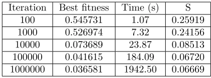
To solve presented examples by NM simplex search method, three initial vertices were generated randomly. Each vertex is considered a real valued vector by 20 entries. So each vertex estimates unknownq(t), and each entry of vertices estimates q(tj) attj =j×0.05,j = 1,2,3, . . . ,20. To determine unknownq(t), the best vertex is interpolated at the end of algorithm. Tables 6–7 present results of implementation of NM for determine unknownq(t) at Examples 1–3, respectively.
Table 5: The results of 100 to 1000000 iteration for determiningq(t) at Example 1 by implementing NM for three vertices
Iteration Best fitness Time (s) S
100 0.545731 1.07 0.25919
1000 0.526974 7.32 0.24156
Galley
Pro
of
Table 6: The results of 100 to 1000000 iteration for determiningq(t) at Example 2 by implementing NM for three verticesIteration Best fitness Time (s) S
100 0.156634 0.89 0.20997
1000 0.147336 2.87 0.13720
10000 0.099725 17.90 0.08711 100000 0.054095 153.17 0.08124 1000000 0.017139 1626.01 0.02814
Table 7: The results of 100 to 1000000 iteration for determiningq(t) at Example 3 by implementing NM for three vertices
Iteration Best fitness Time (s) S
100 0.115466 0.73 0.19575
1000 0.109927 1.98 0.12761
10000 0.080606 19.36 0.07540 100000 0.044853 113.71 0.07341 1000000 0.012802 1094.75 0.01937
7.3 Solving examples by hybrid algorithm
In this subsection, Examples 1–3 are solved by proposed hybrid algorithm in Section 5. In this algorithm, a population of 10 vectors of 20 entries is used as the initial guess for numerical results. Therefore, each vec-tor estimates unknown q(t) and each entry of vectors estimates q(tj) at
Galley
Pro
of
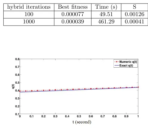
Table 8: The results of 100 to 1000 iteration for determining q(t) at Example 1 by implementing hybrid algorithm for ten verticeshybrid iterations Best fitness Time (s) S
100 0.000077 49.51 0.00126
1000 0.000039 461.29 0.00041
Figure 5: Exact and numericq(t) for 1000 iterations by implementing hybrid algorithm at Example 1
Table 9: The results of 100 to 1000 iteration for determining q(t) at Example 2 by implementing hybrid algorithm for ten vertices
Hybrid iterations Best fitness Time (s) S
100 0.000105 41.78 0.00212
1000 0.000028 436.22 0.00038
Table 10: The results of 100 to 1000 iteration for determiningq(t) at Example 3 by implementing hybrid algorithm for ten vertices
Hybrid iterations Best fitness Time (s) S
100 0.000063 37.19 0.00092
Galley
Pro
of
Figure 6: Exact and numericq(t) for 1000 iterations by implementing hybrid algorithm at Example 2Figure 7: Exact and numericq(t) for 1000 iterations by implementing hybrid algorithm at Example 3
7.4 Comparison
Galley
Pro
of
has created, exploitation of NM and exploration of GA caused that accuracy improve. As total error of hybrid algorithm for 100 and 1000 iterations be-came better in comparison with the NM and GA performance with almost the same execute time.Figure 8: Values of total error(S) for different numbers of iterations by implementing NM and GA at Example 1
Galley
Pro
of
Figure 10: Values of total error(s) for different numbers of iterations by implementing NM and GA at Example38 Conclusion
A numerical method to estimate unknown boundary condition is proposed for these kinds of NIPPs, and the following results are obtained:
1. The present study successfully applies the numerical method to NIPPs.
2. To solve the NIPPs by GA, NM, and hybrid algorithm, the unknown function will be guessed and we do not need the regularization. This will improve the execution time.
3. This hybrid algorithm is able to combine whit every direct solution methods.
4. This method does not need to powerful mathematic base.
5. Acceptable accuracy and execute time at the hybrid algorithm.
References
1. Babolian, E. and Saeidian, J. Analytic approximate solutions to Burg-ers, Fisher, Huxley equations and two combined forms of these equations, Commun. Nonlinear Sci. Numer. Simulat., 14 (2009), 1984–1992.
Galley
Pro
of
3. Cant´u-Paz, E. A Summary of Research on Parallel Genetic Algorithms,IlliGAL Report No 95007, University of Illinois, 1995.
4. Chiwiacowsky, L.D., de Campos Velho, H.F., Preto, A.J., and Stephany, S. Identifying initial condition in heat conduction transfer by a genetic algorithm: a parallel approach, in: 24th Iberian Latin American Congress on Computational Methods in Engineering, Ouro Preto, Brazil, 2003.
5. Holland, J.H. Adaptation in Natural and Artificial System, University of Michigan Press, Ann Arbor, 1975.
6. Katari, V., Malireddi, S., and Srujan Kollisetty, V.N.K.,An efficient hy-brid algorithm for data clustering using improved genetic algorithm and Nelder Mead simplex search, International Conference on Computational Intelligence and Multimedia Applications, 2007.
7. Levine, D. A parallel genetic algorithm for the set partitioning problems, Mathematics and Computer Science Division, Argone National Labora-tory Rept., University of Illinois, 1994.
8. Liu, F.-B.A modified genetic algorithm for solving the inverse heat transfer problem of estimating plan heat source, Int. J. Heat and Mass Transfer, 51 (2008), 3745–3752.
9. Nelder, J. A. and Mead, R.A simplex method for function minimization, Comput. J. 7 (1965), no. 4, 308–313.
10. Olsson, D. M. and Nelson, L. S.The Nelder–Mead simplex procedure for function minimization, Technometrics, 7 (1965) 308–313.
11. Pourgholi, R., Tavallaei, N., and Foadian, S. application of Haar basis method for solving some ill-posed inverse problems, J. Math. Chem., 8(50) (2012), 2317–2337.
12. Shahrezaee, A. M. and Hoseini nia, M.Solution of Some Parabolic Inverse Problems by Adomian Decomposition Method, Appl. Math. Sci., 5(50) (2011), 3949–3958.
13. Sharapov R. R. and Lapshin A. V.Convergence of Genetic Algorithms, Pattern Recognition and Image Analysis, 16(3) (2006), 392–397.
14. Spendley, W., Hext, G. R., and Himsworth, F. R.Sequential application of simplex designs in optimization and evolutionary operation. Technomet-rics, 4(4) (1962), 441–461.
15. Mckinnon K. I. M. Convergence of the Nelder–Mead simplex method to a nonstationary point, SIAM J. Optim., 9(1) (1998), 148–158.
Galley
Pro
of
17. Walsh, G. R.An Introduction to Linear Programming, ISBNﻞﺋﺎﺴﻣ ﻞﺣ یاﺮﺑ ﺪﯿﻣ -رﺪﻠﻧ یﻮﺠﺘﺴﺟ شور و ﮏﯿﺘﻧژ ﻢﺘﯾرﻮﮕﻟا سﺎﺳا ﺮﺑ ارﺎﮐ ﯽﺒﯿﮐﺮﺗ ﻢﺘﯾرﻮﮕﻟا ﮏﯾ ﯽﻄﺧﺮﯿﻏ یﻮﻤﻬﺳ سﻮﮑﻌﻣ
ﯽﻠﻗرﻮﭘ ﺎﺿر و ﻪﻋرﺰﻣ ﺎﻧاد ﻦﺴﺣ
ﺮﺗﻮﯿﭙﻣﺎﮐ مﻮﻠﻋ و ﯽﺿﺎﯾر هﺪﮑﺸﻧاد ،نﺎﻐﻣاد هﺎﮕﺸﻧاد
١٣٩٧ دادﺮﺧ ٢٣ ﻪﻟﺎﻘﻣ شﺮﯾﺬﭘ ،١٣٩۶ رذآ ۴ هﺪﺷ حﻼﺻا ﻪﻟﺎﻘﻣ ﺖﻓﺎﯾرد ،١٣٩۶ ﺖﺸﻬﺒﯾدرا ١۵ ﻪﻟﺎﻘﻣ ﺖﻓﺎﯾرد
-رﺪﻠﻧ ﺲﮑﻠﭙﻤﯿﺳ یﻮﺠﺘﺴﺟ شور و ﮏﯿﺘﻧژ ﻢﺘﯾرﻮﮕﻟا سﺎﺳا ﺮﺑ ﯽﺒﯿﮐﺮﺗ ﻢﺘﯾرﻮﮕﻟا ﮏﯾ ،ﻪﻟﺎﻘﻣ ﻦﯾا رد: هﺪﯿﮑﭼ .دﻮﺷ ﯽﻣ ﺐﯿﮐﺮﺗ ﯽﻄﺧ ﺮﯿﻏ سﻮﮑﻌﻣ یﻮﻤﻬﺳ ﻞﯾﺎﺴﻣ رد تراﺮﺣ ﻪﺟرد ﻦﯿﯿﻌﺗ یاﺮﺑ تﺎﻌﺑﺮﻣ ﻦﯾﺮﺘﻤﮐ شور ﺎﺑ ﺪﯿﻣ ﺞﯾﺎﺘﻧ .دﺮﯿﮔ ﯽﻣ راﺮﻗ ﺪﯿﯾﺎﺗ درﻮﻣ یﻮﻤﻬﺳ ﯽﻄﺧﺮﯿﻏ سﻮﮑﻌﻣ ﻞﺋﺎﺴﻣ زا لﺎﺜﻣ ﺪﻨﭼ ﺎﺑ ﯽﺒﯿﮐﺮﺗ ﻢﺘﯾرﻮﮕﻟا ﯽﯾارﺎﮐ رﻮﻃ ﻪﺑ ﺪﯿﻣ -رﺪﻠﻧ ﺲﮑﻠﭙﻤﯿﺳ یﻮﺠﺘﺴﺟ شور و ﮏﯿﺘﻧژ ﻢﺘﯾرﻮﮕﻟا زا ﺮﺘﻬﺑ ،ﯽﺒﯿﮐﺮﺗ شور ﻦﯾا ﻪﮐ ﺪﻫد ﯽﻣ نﺎﺸﻧ ﺖﻋﺮﺳ ﺎﺑ یا ﻪﺘﺴﻫ ﮏﺗ هﺪﻧزادﺮﭘ ﮏﯾ رد هﺪﺷ حﺮﻄﻣ یﺎﻫ ﻢﺘﯾرﻮﮕﻟا یزﺎﺳ هدﺎﯿﭘ ﺎﺑ یدﺪﻋ ﺞﯾﺎﺘﻧ .ﺖﺳا ﻪﻧﺎﮔاﺪﺟ .ﺖﺳا هﺪﻣآ ﺖﺳﺪﺑ GHz ٢٬٢٠