Pole Assignment Of Linear Discrete-Time Periodic Systems In Specified Discs Through State Feedback

*Corresponding Author, Email: [email protected]



Pole Assignment Of Linear Discrete-Time Periodic

Systems In Specified Discs Through State Feedback

H. A. Tehrani*

Assistant Professor, Department of Mathematics, Shahrood University, Shahrood, Iran

ABSTRACT

The problem of pole assignment, also known as an eigenvalue assignment, in linear discrete-time

periodic systems in discs was solved by a novel method which employs elementary similarity operations.

The former methods tried to assign the points inside the unit circle while preserving the stability of the

discrete time periodic system. Nevertheless, now we can obtain the location of eigenvalues in the specified

discs, randomly. An illustrative example with random system matrices is presented in order to show the

effectiveness of the method.

KEYWORDS

:

1. INTRODUCTION

The study of discrete-time periodic systems has received considerable attention in recent years by many authors; for example, see [1,5-7,11,17-20]. Aliev et al. [1] used a gradient free method, where the cost function for the discrete-time case was minimized. Farges [5] introduced an LMI method to this problem. In the frequency domain, the parametric transfer function (Lampe and Rossenwasser [15], Lampe et al. [16]), the harmonic analysis (Zhou and Hagiwara [20]) and the lifting based methods (Varga [19]) have also been proposed. Moreover, Both norm-bounded uncertainty and polytopic uncertainty have been discussed by Souza and Trono [18], regarding the stabilization problem of the linear discrete-time periodic (LDP) systems. Furthermore, the H2 norm of the LDP systems with polytopic uncertainties has been illustrated by Farges et al. [6]. In many applications, mere stability of the controlled object is not enough, and it is required that the poles of the closed-loop system lie in a restricted region of stability. Several design methods have been proposed which utilize the LQ technique to allocate for the desired pole. Amin [2] found an improved result, whereas the optimality of the closed-loop system was assured. Furuta and Kim [9] obtained a method for assigning the closed loop poles to a specified disc based on gain and phase margins which named -stability margin. They considered the condition in which the perturbations are unknown gains as a diagonal form. Figueroa and Romagnoli [8] presented a method for designing the controllers which attempt to place the roots of a characteristic polynomial of an uncertain system inside some desired regions. The analysis is based on the transfer function of a characteristic polynomial. Chou [4] described another pole assignment method with a spectral radius and proposed a pulse transfer function. Its procedure is simple, but it is used only for checking the positions of the closed loop poles, not for designing the controller. Benner and Castillo and Quintana-Orti [3] worked on a method for the partial stabilization of large-scale discrete-time linear control systems. Recently, Grammont and Largillier [10] used an approach to localize the matrix eigenvalues in a way that they build an appropriate small neighborhood for each eigenvalue (or for a cluster).

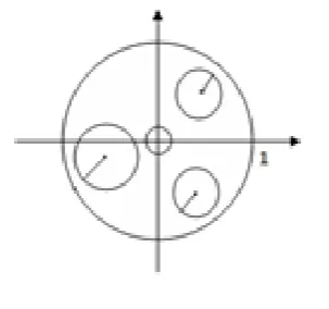
A well-known desired region for the discrete systems is a disc D(c,r)centered at (c,0)with the radius r, in whichcr1, as shown in Fig. 1. In this paper, our porpose is to present a method for the localization of

plane through state feedback control for the linear discrete-time periodic control systems.

Fig. 1.Specified discs inside a unit circle

2. PROBLEM STATEMENT

Consider the linear discrete-time periodic system of the form

k k k k

k Ax Bu

x _1 

(1)

where the matrices

A

_k



n n and

B

_k



n m are periodic with period ofK1, i.e.,

A

k K



A B

k

,

k K



B

k. Suppose the periodic

matrix pair

(

A B

_k

,

_k

)

are completely reachable [6,20], then the problem of time-optimal control of the periodic system lead us to find the periodic feedback matrices

m n k

F



 in a way that the poles of the monodromy matrix

) (

. . . ) (

) 0 ,

(K A_{K 1} B_{K 1}F_{K 1} A₀ B₀F₀ BF

A   

    

(2)

are located at the origin of the complex plane. The state transition matrix of (1) is defined by [16]

  

  



 

 A A A t r

A

r t I

r t

r r t

t 1 2... 1

: ) , (

) , (t r

 undefined for tr

It is clear that (tK,rK)(t,r), tr due to the periodicity of Ak_{. The matrix}

1 ..., , 1 , 0 ), , (

:   

_r r Kr r K

, is known as the monodromy matrix of (1) at the time

r

. The eigenvalues of r_{, are known as the characteristic multipliers of (1).}

They are independent of

r

. In other words, all r_{s have}

multipliers lie inside the unit circle. The reachability grammian matrix of (A(.),B(.)) is given by



 



_{  }

 

 1 (, 1) (, 1), :

) , (

t r j

j j

s t r t j B B t j t r

W

₍₃₎

Various system properties such as controllability, observability, stabilizability, detectability can be defined just for the time-invariant case [11,19]. A stabilizability criterion is that the system (1) or the periodic pair

(.)) (.),

(A B is stabilizable at the time

r

if and only if the pair (r,Ws(rK,r)) is stabilizable.

Note that the poles of the intermediate closed-loop systems, _i A_iB_iF_i, for i1,...,K1 may be assigned to any set of eigenvalue spectrum



1,2,...,n





 in a unit disc such that the

controllability of the final pair ( , 0) 1

1 0 1

1

B

A i

K i i K i





_



   

is preserved [7,12,13].

We call the pairs (Ai,Bi) for i1,...,K1 the

intermediate systems, and treat them as individual standard systems. In this paper, we present an efficient approach for the localization of eigenvalues in small specified regions for the linear discrete-time periodic systems. The procedure has two stages. We first consider the pairs (A_i,B_i) for i1,...,K1 and obtain a state feedback matrix F_i which assigns all the eigenvalues of the closed-loop system _i for i1,...,K1 inside the unit circle centered at the origin, then for the final pair

) ,

( 0

1 1 0 1

1

B

A i

K i i K i





_



  

 , a state feedback matrix F0 which

assigns all the closed-loop system eigenvalues in a small specified disc or discs is found. Since

0 0

0 0 1 1

1 )...( )

( ) 0 ,

(K A_K B_K F_K A BF A BF BF

A     

 _{   }

(4)

where 0 1

1

A

A i

K i

 

_

 

, 0

1 1

B

B i

K i

 

_

 

and whereas we assign all the closed-loop system eigenvalues in a small specified disc or discs, therefore all of the monodromy matrix eigenvalues are located in a small specified disc or discs.

3. POLE (EIGENVALUE)ASSIGNMENT INSIDE ADISC

Consider a controllable linear time-invariant standard discrete-time system defined by this state equation

) ( ) ( ) 1

(k Axk Bu k

x   

(5)

where xn, um and the matrices A and B are real constant matrices of appropriate dimensions with

m B

rank( ) . The Kronecker invariants, p_i, i1,...,m

[12] are defined to be regular if the difference between any of them is not greater than one. We define control low of the form

) ( ) (k Fxk

u 

₍₆₎

Consider the state transformation

 

t Tx

 

t

x  ~

(7)

where T can be obtained through elementary similar operations as described in [12]. In this way,

AT T

A~ 1 and B~T1B are in a compact canonical form, known as vector companion form:

  

 

  

  

 

m n m m

n I

G A

0 ___ __________

~ 0

 



 

  

  

 m m n

B B

0 _______

~ 0

(8)

Here,

G

₀ is an

m n



matrix and is an

m m



upper triangular matrix. Note that if the Kronecker invariants of the pair



B A

,



are regular, then

A

and

B

are always in the above form [12]. In the case of irregular Kronecker invariants, some rows of

I

_{n m} in

A

are displaced [13]. It may also be concluded that if the vector companion form of A~ obtained from the similar operations has the above structure, then the Kronecker invariants associated with the pair



B A

,



are regular [12].

The state feedback matrix which assigns all the eigenvalues to zero, for the transformed pair

 

B A

,

, it is then chosen as

x F x G B

u ₀1 ₀~~_p~

(9)

Which results in the primary state feedback matrix for the pair



B,A



defined as

1

~ 

FT

F_{p p}

(10)

The transformed closed-loop matrix A BFp

~ ~ ~ ~

0 



                m m n m n n m I 0 ___ __________ 0 ~ 0 

(11)

Theorem 1: Let D be a block diagonal matrix in the form              k D D D D        0 0 0 0 0 0 2 1

(12)

where each D_j ,(j1,2,...,k)is either in the form of

        j j j j j D    

(13)

(to designate the complex conjugate eigenvalues  j ij

) or in case of real eigenvalues

] [ j

j d

D 

(14)

If such a block diagonal matrix D with self conjugate eigenvalue spectrum is added to the transformed closed-loop matrix, ~₀, then the eigenvalues of the resulting matrix are exactly the same as the eigenvalues in the spectrum.

Proof: The primary compact Jordan form in the case of regular Kronecker invariants is in the form

                m m n m n n m I 0 ___ __________ 0 ~ 0 

(15)

The sum of ~₀ with D has the form:

D

H~ ~₀ 

(16)

                          k m m n m n n m D D I       0 0 0 ___ __________ 0 ₁

(17)

                        k r l l D I D I D D D                      0 0 0 0 0 0 0 0 0 0 0 0 0 0 0 0 0 0 0 0 1 1 2 1

(18)

where Is, s1,2,...,r are the unit matrices of size 2 in

case nm is even. In case nm is odd, only one I_s

takes the form of a unit matrix of size one.

By expanding det(H~I) along the first row, it is obvious that the eigenvalues of H~ are the same as the eigenvalues of D. For the case of irregular Kronecker invariants [13], only some of the unit columns of I_nm

are displaced. Since the unit elements are always below the main diagonal, the proof is applied in the same manner (H 0D

~ ~

remains in a lower triangular block matrix in any case).

4. COROLLARY

A matrix H~_, with similar structure as A~ , can be obtained from H~ by performing elementary similar operations

) ( )

(j Column i

Column j

(19)

followed by

) ( )

(i Row j

Row j

(20)

For jn,n1,,m ijm

Hence, the matrix H~_thus obtained will be in the primary vector companion form such that:

            

m n m m

n I H H 0 ___ __________ ~ 0  

(21)

where H₀ is an mn matrix [14] .

Because of the similar operations, the eigenvalues of the matrix H~_ are the same as the eigenvalues of H~ and also that ofD. Now the feedback matrix of the pair

) ~ , ~

(A B is defined by:

) ( ~ ~ 0 0 1 0 0 1

0 H B G H

B F

F _p     

(22)

Theorem 2: The state feedback matrix K~ assigns the eigenvalues of the closed-loop matrix ~A~B~K~ inside a circle with center

c

and radius

r

. If the circle intersects axis of abscissas, we suppose j,j to be in the form of:

) Re( ) 1 , 0 ( * ) ) Im(

(r2 c 2 random c

sqrt  



) 1 , 0 ( *

) ) Im( ) (

(sqrt r2 l2 c random

j   



(24)

and if the circle doesn’t intersect axis of abscissas, we suppose

) Re( ) 1 , 0 (

*random c

r

j  



(25)

) Im( ) 1 , 0 ( )

(r2 l2 random c

sqrt

j    



(26)

where we take lj Re(c) if j*Re(c)0,

otherwise, lj Re(c) .

For assigning real valued eigenvalues inside a circle with center c and radius r, we choose

) Re( ) 1 , 0 ( *

) ) Im(

(r2 c 2 random c

sqrt

dj   

(27)

Proof: The eigenvalues of matrix D defined above fall inside a circle with center c and radius r.

Let



( )



0 0 ~

~ ~ ~

0 0 1 0 , 0 , 0

H G B B

I G K

B A

m m n m m n m n

            

    

 

  

(28)

or

   

 

     

 

  

 

 

 

 

m m n m

n

m m n m

n

I H I

H B B G B B G

, 0

, 0 1 0 0 0 1 0 0 0

0

0 ~

(29)

Clearly, H

~ ~_

 _{, since} H~_{is similar to the matrix}

H~_{and the eigenvalues of matrix} H~_{are the same as that}

of matrix Dand elementary similar operations do not change the eigenvalues, then the eigenvalues of the closed-loop matrix ~A~B~F~ fall inside a circle with center

c

and radius

r

.

Remark: Since K~ assigns the eigenvalues of the closed-loop matrix ~A~B~F~ inside a circle with center

c

_{and radius}

r

, it is obvious that the state feedback

controller matrix,

1 0 0 1 0 1

) (

~  _  _{ } 

FT B G H T

F _also

assigns the eigenvalues of the closed-loop matrix

BF A 

 _{inside a circle with center}

c

_{and radius}

r

, too.

Note that for assigning the eigenvalues of the closed-loop matrix in a specified spectrum 



1,2,,n



_{, it}

was supposed that:

n j

Dj j 1,2,,

(30)

5. AN ALGORITHM FOR ASSIGNMENT OF

EIGENVALUES INSIDE ADISC

D

(

c

,

r

)

.

In this section, we first give an algorithm for finding a state feedback matrix which assigns zero eigenvalues to the closed-loop system. Then we determine a gain matrix which assigns the closed-loop eigenvalues inside a circle with center

c

and radius

r

.

Input: The controllable pair(A,B), the primary state feedback F_p, B₀1and T1which are calculated by the algorithm proposed by Karbassi and Bell [12,13], the center cand radius rof the target circle.

Step 1. Construct the block diagonal matrix D in the form (12), in which for assigning complex valued eigenvalues inside the circle with center cand radius r, if circle intersects the axis of abscissas, we take

) Re( ) 1 , 0 ( *

) ) Im(

(r2 c 2 random c

sqrt

j  



) 1 , 0 ( *

) ) Im( ) (

(sqrt r2 l2 c random

j  



Otherwise, we choose

) Re( ) 1 , 0 (

*random c r

j 



) Im( ) 1 , 0 ( )

) ) Re( (

(r2 c 2 random c

sqrt _j

j      



where lj Re(c) if j*Re(c)0 or

) Re(c

lj  if j*Re(c)0

For the real valued eigenvalues inside the circle with center

c

and radius

r

, we choose

) Re( ) 1 , 0 ( *

) ) Im(

(r2 c2 random c

sqrt

d_j  

Step 2. Set H0D ~ ~

Step 3. Transform H~ to primary vector companion form H~_as in (21) using elementary similar operations as specified in corollary of theorem 1.

step 4. Now, compute

1 0 1 0

 

 F B HT

F _p

.

6. ILLUSTRATIVE EXAMPLE

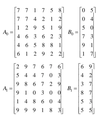
                     2 2 9 2 1 6 1 8 8 5 6 4 3 2 6 3 6 4 9 1 5 9 2 1 2 1 2 4 7 7 8 5 7 1 7 7 0 A                      7 1 1 9 3 7 0 5 4 0 5 0 0 B                      3 8 1 9 9 9 4 0 6 8 4 1 0 0 3 0 1 9 9 2 7 6 8 9 3 0 7 4 4 5 6 7 6 7 9 2 1 A                      5 5 3 5 7 8 7 3 2 4 9 6 1 B

The open loop monodromy matrix eigenvalues are:

}

17

.

0

,

22

.

18

10

.

8

,

30

.

21

15

.

38

,

081

.

81

{





i



i



which are widely spread in the complex plane. In order to locate them in small discs inside the unit circle, we utilize the above algorithm step by step. First, we obtain a state feedback matrix F₁ which assigns all the eigenvalues of the closed-loop system ₁A₁B₁F₁ inside the unit circle centered at the origin. By using the algorithm, the state feedback matrix obtained is:

             0803 . 2 9747 . 1 1785 . 2 7247 . 2 3675 . 2 1034 . 5 2480 . 1 7960 . 1 2410 . 1 5845 . 1 3539 . 1 3142 . 7 1 F

It can be verified that the closed-loop eigenvalues are



0.83180.2791i,0.68130.2778i,0.4289,0.7095



Now we consider A₁A₀ and B₁B₀ and we find the state feedback matrix F0which assigns the

eigenvalues of the closed-loop system ABF₀ inside the discs: ) 2 . 0 , 0 ( ), 3 . 0 , 1 . 0 6 . 0 ( ), 2 . 0 , 5 . 0 5 . 0 ( ), 2 . 0 , 5 . 0 5 . 0 ( 4 3 2 1 D i D i D i D    

By using the algorithm, the state feedback matrix obtained is:                    6705 . 1 2057 . 1 4148 . 1 4796 . 0 5911 . 1 6417 . 1 2842 . 0 3519 . 0 6597 . 0 1959 . 1 4837 . 0 2434 . 0 0 F

The closed-loop monodromy eigenvalues are now:



0.56090.5361i,0.06060.1032i,0.65470.1330i



which are inside the specified above the discs as shown in the following figure:

Fig. 2.Poles inside the prescribed discs

7. CONCLUSION

The problem of pole assignment, also known as an eigenvalue assignment, in linear discrete-time periodic systems in specified discs inside the unit circle, was achieved by implementation of the elementary similar operations proposed by Karbassi and Tehrani [14], assigning the closed-loop system eigenvalues randomly inside the prescribed discs. The main advantage of this technique is the ease by which the algorithm can be implemented. Although it is claimed that similar operations inherit numerical errors, generically they work as good as other robust numerical algorithms. The numerical example, which was tested, showed that the algorithm works perfectly, although the system matrices and the location of the discs were chosen randomly. The case of pole assignment for the linear discrete-time periodic systems through output feedback is to be considered in the future.

REFERENCES

[1] F.A. Aliev, C.C. Arcasoy, V.B. Larin, and N.A. Safarova, “Synthesis problem for periodic systems by static output feedback,” Applied and Computational Mathematics. vol 4(2),pp. 102– 113, 2005.

[2] F.A. Aliev, C.C. Arcasoy, V.B. Larin, and N.A. Safarova, “Synthesis problem for periodic systems by static output feedback,” Applied and Computational Mathematics. vol 4(2),pp. 102– 113, 2005.

[4] J. H. Chou, “Pole assignment robustness in a specified disk,” Systems & Control Letters, vol 16, pp. 41-44, 1991.

[5] C. Farges, D. Peaucelle, and D. Arzelier,” Resilient static output feedback stabilization of linear periodic systems,” In: 5th IFAC Symposium on Robust Control Design, Toulouse 2006. [6] C. Farges, D. Peaucelle, D. Arzelier, and J.

Daafouz, “Robust performance analysis and synthesis of linear polytopic discrete-time periodic systems via LMIs,” Systems & Control Letters, vol 56(2), pp. 159.166, 2007.

[7] M. M. Fateh, H. Ahsani Tehrani, and S. M. Karbassi, “Repetitive control of electrically driven robot manipulators,” International Journal of Systems Science, Published Online: 18 Oct 2011. [8] J. L. Figueroa and J. A. Romagnoli, “An algorithm

for robust pole assignment via polynomial approach,” IEEE Transactions on Automatic Control, vol 39,pp. 831-835,1994.

[9] K. Furuta and S. B. Kim, “Pole assignment in a specified disk,” IEEE Transactions on Automatic Control, vol 32, pp. 423-427, 1987.

[10] L. Grammont and A. Largillier, “Krylov method revisited with an application to the localization of eigenvalues ,” Numerical Functional Analysis and Optimization, vol 27, pp. 583-618,

[11] G. Guo, J.F. Qiao, and C.Z. Han, “Controllability of periodic systems: continuous and discrete,” in proc IEE Control Theory and Applications, vol 151, pp. 488-490, 2004.

[12] S.M. Karbassi and D.J. Bell, “Parametric time-optimal control of linear discrete-time systems by state feedback-Part 1: Regular Kronecker invariants,” International Journal of Control, vol. 57, pp. 817-830, 1993.

[13] S.M. Karbassi and D.J. Bell, “Parametric time-optimal control of linear discrete-time systems by state feedback-Part 2: Irregular Kronecker invariants,” International Journal of Control, vol 57, pp. 831-839,1993.

[14] S.M. Karbassi and H.A. Tehrani, “Parameterizations of the state feedback controllers for linear multivariable systems ,” Computers and Mathematics with Applications, vol 44, pp. 1057-1065, 2002.

[15] B.P. Lampe and E. N. Rossenwasser, “Closed formulae for the L2-norm of linear continuous-time periodic systems ,” In: Proc. PSYCO, 231-236, Japan 2004.

[16] B.P. Lampe, M. A. Obraztso, and E. N. Rosenwasser, “Statistical analysis of stable

FDLCP systems by parametric transfer matrices ,” International Journal of Control, vol 78(10), pp. 747-761, 2005.

[17] S. Longhi, and R. Zulli, “A note on robust pole assignment for periodic systems,” IEEE Transactions on Automatic Control, vol 41, pp. 1493-1497, 1996.

[18] C.E.De. Souza and A. Trono, “An LMI approach to stabilization of linear discrete-time periodic systems,” International Journal of Control, vol 73, pp. 696-703, 2000.

[19] A. Varga, “Computation of l-infinity norm of linear discrete-time periodic systems,” In: Proc. MTNS 2006.