On a novel modification of the Legendre collocation method for
solv-ing fractional diffusion equation
Hosein Jaleb
Department of Mathematics, Central Tehran Branch, Islamic Azad University, Tehran, Iran.
E-mail: [email protected]
Hojatollah Adibi∗
Department of Applied Mathematics,
Faculty of Mathematics and Computer Science, Amirkabir University Of Technology, Tehran, Iran. E-mail: [email protected]
Abstract In this paper, a modification of the Legendre collocation method is used for solving the space fractional differential equations. The fractional derivative is considered in the Caputo sense along with the finite difference and Legendre collocation schemes. The numerical results obtained by this method have been compared with other methods. The results show the capability and efficiency of the proposed method.
Keywords. Fractional diffusion equation, Caputo derivative, Fractional Riccati differential equation,
Fi-nite difference, Collocation, Legendre polynomials.
2010 Mathematics Subject Classification. 34A08.
1. Introduction
The fractional partial differential equations (FPDEs) are used in numerous prob-lems of physics, engineering, chemistry, mathematics, biology, and viscoelasticity [1,
15, 19, 22]. Most fractional differential equations suffer from lacking of exact ana-lytical solutions. So many authors are seeking ways to numerically solve these prob-lems [4, 25].
Recently, some different methods for solving fractional differential equations have been given such as variational iteration method [7], homotopy perturbation method [23], adomian decomposition method [8], homotopy analysis method [6], and collocation method [21]. A least square finite element solution of a fractional-order two-point boundary value problems, has been studied in [5]. Sumudu transform method for solving fractional differential equations and fractional diffusion-wave equation as well proposed in [3]. Wavelet operational method for solving fractional partial differential equations used in [18]. Method of lines to transform the space fractional Fokker-Planck equation into a system of ordinary differential equations studied in [13, 14]. The space fractional diffusion equations are solved numerically. Khader used Legendre
Received: 20 January 2019 ; Accepted: 23 February 2019.
∗Corresponding author.
collocation method to discretize space fractional diffusion equations to obtain a linear system of ordinary differential equations and he solved the resulting system by finite difference method [10]. Dehghan and et al. [24] proposed Tau approach to solve space fractional diffusion equations.
2. Preliminary ideas and definitions
Definition 2.1. The Caputo fractional derivative operator C
0Dαx of orderαis de-fined in the following form [22]:
C
0Dαxf(x) = 1 Γ(m−α)
Rx 0
f(m)(t)
(x−t)α−m+1dt, α >0,
wherem−1< α≤m, m∈N, x >0.
Caputo fractional derivative operator is a linear operation and for the Caputo derivative we have [11]:
C 0D
α
xc= 0, (2.1)
C 0D
α xx
n = (
0, n∈N0 and n <dαe, Γ(n+1)
Γ(n+1−α)x
n−α, n∈N
0 and n≥ dαe,
(2.2)
where cis a constant and dαe denotes the smallest integer greater than or equal to
αandN0={0,1,2, . . .}.Forα∈N0,the Caputo differential operator coincides with the classic differential of integer order ( [9,11,20]).
Definition 2.2. Theweighted−LPnormis defined in the following form [2]:
kukLpw(−1,1)= (
Z 1
−1
|u(x)|pw(x)dx)1/pf or 1≤p <∞, (2.3)
where we also have
kukL∞
w(−1,1)= sup
−1≤x≤1
|u(x)|=kukL∞(−1,1). (2.4)
Definition 2.3. We define natural Sobolev norms as follows [2]:
kukHm
w(−1,1)= (
m X
k=0
ku(k)k2 L2
w(−1,1))
1/2. (2.5)
The Hilbert space associated with this norm is denoted byHm
w(−1,1).We also define the seminorms
|u|Hm,N
w (−1,1)= (
m X
k=min(m,N+1)
ku(k)k2 L2
w(−1,1))
1/2. (2.6)
2.2. A brief review of the Legendre polynomials
The well known Legendre polynomials are defined on the interval [-1, 1] as [10]
L0(z) = 1,
L1(z) =z,
Lk+1(z) = 2k+ 1
k+ 1zLk(z)−
k
k+ 1Lk−1(z), k= 1,2, . . . . (2.7)
It is often more useful to utilize some other Legendre polynomials introduced next. In order to use such polynomials on the intervalx∈[0,1], we define the so called shifted Legendre polynomials by introducing the change of variablez = 2x−1. We denote the shifted Legendre polynomialsLk(2x−1) by Pk∗(x), thenPk∗(x) can be obtained as follows:
Pk∗+1(x) = (2k+ 1)(2x−1) (k+ 1) P
∗ k(x)−
k k+ 1P
∗
k−1(x), k= 1,2, ..., (2.8)
whereP0∗(x) = 1 and P1∗(x) = 2x−1. The Legendre polynomialsPk∗(x) of degree k is given by the following:
Pk∗(x) = k X
i=0
(−1)k+i(k+i)!xi
(k−i)(i!)2 , (2.9)
wherePk∗(0) = (−1)k and Pk∗(1) = 1. The orthogonality condition is
Z 1
0
Pi∗(x)Pj∗(x)dx=
1
2i+1, i=j
A function y(x), which is square integrable in [0,1], may be expressed in terms of shifted Legendre polynomials as
y(x) = ∞ X
i=0
yiPi∗(x),
where
yi= (2i+ 1) Z 1
0
y(x)Pi∗(x)dx, i= 1,2, . . . . (2.11)
In practice, only the first (m+1)-terms of shifted Legendre polynomials are considered. If so, we have
ym(x) = m X
i=0
yiPi∗(x). (2.12)
Theorem 2.1. Lety(x) be approximated by shifted Legendre polynomials as Eq. (2.12) and also supposeα >0,then [11]
C 0D
α
x(ym(x)) = m X
i=dαe i X
k=dαe
yiw (α) i,kx
k−α, (2.13)
wherew(i,kα) is given by
wi,k(α)= (−1)
(i+k)(i+k)!
(i−k)!(k)!Γ(k+ 1−α). (2.14)
3. The proposed method
We consider space fractional diffusion equation
∂u(x, t)
∂t =d(x, t)
∂αu(x, t)
∂xα +s(x, t), (3.1)
a < x < b, 0≤t≤M, 1< α≤2,
with initial condition
u(x,0) =u0(x), a < x < b, (3.2)
and boundary conditions
where the functions(x, t) is a source term.
We apply the Legendre collocation method to discretize Eq. (3.1) and to get a linear system of ordinary differential equations and use the finite difference method (FDM) [16, 17] to solve the resulting system, and obtain the coefficients in the ap-proximate solution. If so,u(x, t) is approximated by
um(x, t) = m X
i=0
λi(t)Pi∗(x). (3.4)
Now from Eqs. (3.1), (3.2) and using Theorem 2.1 we have
m X
i=0
dλi(t)
dt P
∗
i(x) =d(x, t) m X
i=dαe i X
k=dαe
λi(t)w(i,kα)xk−α+s(x, t). (3.5)
Collocating, Eq. (3.5) at (m+ 1− dαe) pointsxp yields
m X
i=0
dλi(t)
dt P
∗
i(xp) =d(xp, t) m X
i=dαe i X
k=dαe
λi(t)w(i,kα)xk−αp +s(xp, t), (3.6)
p= 0,1, ..., m− dαe.
Now we take advantage of roots of shifted Legendre Polynomials Pm∗+1−dαe(x) as suitable collocation points.
By substituting Eqs.(3.4) and (2.13) into the boundary conditions (3.3) we get
m X
i=0
Pi∗(a)λi(t) = 0,
m X
i=0
Pi∗(b)λi(t) = 0. (3.7)
If so,dαeequations obtained from (3.7), along with m+1-dαeequations obtained from (3.6) give (m+1) ordinary differential equations which may be solved by using FDM, i=0,1,...,N,τ = MN, 0 ≤ ti ≤M, ti =iτ, to get the m unknownλi, i=0,1,...,m, in various time levelstn. By determining the unknownsλi(tn), the approximate m de-gree polynomials at different time oftn are obtained as follows:
um(x, tn) = m X
i=0
λi(tn)Pi∗(x) =λ n
oP0∗(x) +λ n
1P1∗(x) +λ n
2P2∗(x) +...+λ n mPm∗(x)
in which T is the final time andλni =λi(tn),λ´inxi=λniPi∗(x).
Assume that we have accurate valuesuex(x, tn). Now for improving the proposed method, first we consider the following average:
uN ewap(1)(x, tn) = 1
2[uap(x, tn) +uex(x, tn)], (3.9)
as our first approximate solution, whereuexanduapstand for exact and approximate solution of Eq. (3.1) anduN ewap(1) denote the first approximate solution obtained. It can be seen that
|uN ewap(1)(x, tn)−uex(x, tn)|<|uap(x, tn)−uex(x, tn)|. (3.10)
This confirms that in the first stage the approximate solution gets better with respect to Eq. (3.8).
In the second step, we put
uN ewap(2)(x, tn) = 1
2[uN ewap(1)+uex(x, tn)],
it can be seen that
|uN ewap(2)(x, tn)−uex(x, tn)|<|uN ewap(1)(x, tn)−uex(x, tn)|,
this shows that
|uN ewap(2)(x, tn)|<|uN ewap(1)(x, tn)|.
Proceeding further, are can conclude that in the (n-1)-th stage we have
uN ewap(n)(x, tn)< uN ewap(n−1)(x, tn). (3.11)
4. Error analysis and convergence
This section consists of the convergence analysis and getting an upper bound for the error of the proposed method.
Theorem 4.1. The error |ET(m)|=|Dαy(x)−Dαy
m(x)|for the approximation ofDαy(x) byDαy
m(x) has the following upper bound [11]
|ET(m)| ≤ ∞ X
i=m+1
yi( i X
k=dαe k−dαe
X
j=0
θi,j,k)|, (4.1)
where
θi,j,k=
(−1)i+k(i+k)!(2j+ 1) (i−k)!(k)!Γ(k−α+ 1)×
j X
r=0
(−1)j+r(j+r)! (j−r)!(r!)2(k−α+r+ 1).
Theorem 4.2. (Legendre truncation theorem). The truncation erroru(x)−uN(x), where uN(x) = P
N
k=0ckPk∗(x),is the truncated Legendre series of u, satisfies the inequality [2]
ku(x)−uN(x)kLpw(−1,1)≤CN
−m
m X
k=min(m,N+1)
ku(k)kLpw(−1,1), (4.2)
f or1 ≤p <∞, and for all functions uwhose distributional derivatives of order up to m belong toLpw(−1,1),C is a constant and depends onm.
If so, whenN → ∞,we have
0≤limN−→∞(ku(x)−uN(x)kLpw(−1,1))≤
limN−→∞(CN−mPm
k=min(m,N+1)ku (k)k
Lpw(−1,1)).
(4.3)
In the equation (3.14), if max|Pm
k=min(m,N+1)ku (k)k
Lpw(−1,1)| ≤M.Then
lim N−→∞(CN
−m
m X
k=min(m,N+1)
ku(k)kLpw(−1,1)) = 0
.
Now, according to(3.14), and also according to the squeeze theorem, we have
lim
N−→∞(ku(x)−uN(x)kL
p
Right now, to discuss the modified method an error analysis is presented. By using polynomial approximations obtained Eq. (3.8), and considering
P0(x, tn) =um(x, tn) = m X
i=0
λi(tn)Pi∗(x), (4.4)
we have:
|P0(x, tn)−uex(x, tn)| ≤ε0. (4.5)
whereε0is very small amount. Also from
uN ewap(1)(x, tn) = 1
2[um(x, tn) +uex(x, tn)] =P1(tn), (4.6) we have:
|P1(x, tn)−uex(x, tn)| ≤ε1. (4.7)
whereε1is very small amount.
Considering the ties (4.3), (4.4) and (4.5), we have
|P1(x, tn)−uex(x, tn)| ≤ε1⇒ | 1
2[P0(x, tn) +uex(x, tn)]−uex(x, tn)| ≤ε1
⇒ |P0(x, tn)−uex(x, tn)| ≤2ε1≤ε0,
where yield
ε1≤
ε0
2. (4.8)
Next consideringuN ewap(2)(x, tn) = 12[um(x, tn) +uex(x, tn)] =P2(tn) , we have
|P2(x, tn)−uex(x, tn)| ≤ε2⇒ | 1
2[P1(x, tn) +uex(x, tn)]−uex(x, tn)| ≤ε2,
⇒ |P1(x, tn)−uex(x, tn)| ≤2ε2⇒ | 1
2[P0(x, tn) +uex(x, tn)]−uex(x, tn)| ≤2ε2,
which results in
ε2≤
ε0
22, (4.9)
going ahead process, the n-th stage will be as
εn≤
ε0
2n. (4.10)
whereεn is very small amount.
Accordingly we get the following result
|Pn(x, tn)−uex(x, tn)| ≤εn≤
ε0
2n. (4.11)
Now we deduce that
0≤ lim
n→∞(|Pn(x, tn)−uex(x, tn)|)≤n→∞lim(
ε0
2n). (4.12)
Resit now, according to Eq. (4.12) and also the squeeze theorem, we have
lim
n→∞(|Pn(x, tn)−uex(x, tn|) = 0.
This confirms the convergence issue of the method.
Remark 1. The presented method, can also be used for the numerical solution of the fractional Riccati differential equation.
Dαu(t) +u2(t)−1 = 0, t >0,0< α≤1,
with the initial conditionu(0) =u0.
5. Numerical results
Example 5.1. In this example, we consider the fractional Riccati differential equation of the form
with the initial condition
u(0) =u0, (5.2)
and the parameterα,refers to the fractional order of the time derivative. Forα= 1; the Eq. (5.1) is the standard Riccati differential equation
du(t)
dt +u
2(t)−1 = 0,
the exact solution to this equation is
u(t) = e 2t−1
e2t+ 1.
Now by using Eqs. (2.12) and (2.13), withm= 5, the fractional Riccati differential equation (5.1) is transformed to the following approximated form
5 X
i=1 i X
k=1
ciw (α) i,kt
k−α+ ( 5 X
i=0
ciPi∗(t))2−1 = 0, (5.3)
wherew(i,kα)is defined in Eq. (2.14).
Also, the initial condition Eq. (5.2) is given by
5 X
i=0
ci(Pi∗(0)) =u0. (5.4)
We now collocate Eq. (5.3) at (m+ 1− dαe) pointstp as
5 X
i=1 i X
k=1
ciw (α) i,kt
k−α
p + (
5 X
i=0
ciPi∗(tp))
2−1 = 0, p= 0,1,2,3,4. (5.5)
We know thatts
p are the roots of shifted Legendre polynomialP5∗(t), i.e.
t0= 0.5, t1= 0.2307, t2= 0.7692, t3= 0.0469, t4= 0.9530.
By using Eqs. (5.4) and (5.5), we obtain a system of 6 non-linear algebraic equations with unknownsci, i= 0,1, . . . ,5.
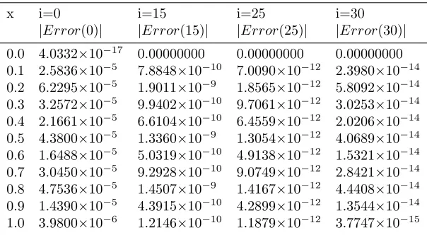
Table 1. Comparison of absolute errors for u(x) at m = 5 with
different values ofifor Example 5.1 by modified method.
x i=0 i=15 i=25 i=30
|Error(0)| |Error(15)| |Error(25)| |Error(30)|
0.0 4.0332×10⁻¹⁷ 0.00000000 0.00000000 0.00000000 0.1 2.5836×10⁻⁵ 7.8848×10⁻¹⁰ 7.0090×10⁻¹² 2.3980×10⁻¹⁴ 0.2 6.2295×10⁻⁵ 1.9011×10⁻⁹ 1.8565×10⁻¹² 5.8092×10⁻¹⁴ 0.3 3.2572×10⁻⁵ 9.9402×10⁻¹⁰ 9.7061×10⁻¹² 3.0253×10⁻¹⁴ 0.4 2.1661×10⁻⁵ 6.6104×10⁻¹⁰ 6.4559×10⁻¹² 2.0206×10⁻¹⁴ 0.5 4.3800×10⁻⁵ 1.3360×10⁻⁹ 1.3054×10⁻¹² 4.0689×10⁻¹⁴ 0.6 1.6488×10⁻⁵ 5.0319×10⁻¹⁰ 4.9138×10⁻¹² 1.5321×10⁻¹⁴ 0.7 3.0450×10⁻⁵ 9.2928×10⁻¹⁰ 9.0749×10⁻¹² 2.8421×10⁻¹⁴ 0.8 4.7536×10⁻⁵ 1.4507×10⁻⁹ 1.4167×10⁻¹² 4.4408×10⁻¹⁴ 0.9 1.4390×10⁻⁵ 4.3915×10⁻¹⁰ 4.2899×10⁻¹² 1.3544×10⁻¹⁴ 1.0 3.9800×10⁻⁶ 1.2146×10⁻¹⁰ 1.1879×10⁻¹² 3.7747×10⁻¹⁵
is obtained via
u5(t) = 5 X
i=0
ciPi∗(t). (5.6)
More specifically forα= 1, Eq. (5.6) gets replaced by
u5(t) = 5 X
i=0
ciPi∗(t) =−4.03323×10⁻¹⁷+ 0.9993x+ (5.7)
0.0157x2−0.4189x3+ 0.1806x4−0.0152x5.
Based upon our method, our results have been compared with the exact solution, in Table 1 and 2. In this tables, errors have been reported for different values ofi.
Example 5.2.In this section, we consider space fractional diffusion equation (3.1) withα= 1.8, of the form [10]
∂u(x, t)
∂t =d(x, t)
∂1.8u(x, t)
∂x1.8 +s(x, t),
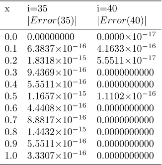
Table 2. Comparison of absolute errors for u(x) at m = 5 with
different values ofifor Example 5.1 by modified method.
x i=35 i=40
|Error(35)| |Error(40)|
0.0 0.00000000 0.0000×10⁻¹⁷ 0.1 6.3837×10⁻¹⁶ 4.1633×10⁻¹⁶ 0.2 1.8318×10⁻¹⁵ 5.5511×10⁻¹⁷ 0.3 9.4369×10⁻¹⁶ 0.0000000000 0.4 5.5511×10⁻¹⁶ 0.0000000000 0.5 1.1657×10⁻¹⁵ 1.1102×10⁻¹⁶ 0.6 4.4408×10⁻¹⁶ 0.0000000000 0.7 8.8817×10⁻¹⁶ 0.0000000000 0.8 1.4432×10⁻¹⁵ 0.0000000000 0.9 5.5511×10⁻¹⁶ 0.0000000000 1.0 3.3307×10⁻¹⁶ 0.0000000000
function: s(x, t) = 3x2(2x−1)e−t. The initial and boundary conditions are respec-tively as
u(x,0) =x2(1−x),
u(0, t) =u(1, t) = 0.
The exact solution of this problem isu(x, t) =x2(1−x)e−t.
We use the present method with m=3, and approximate the solution as follows:
u3(x, t) = 3 X
i=0
λi(t)Pi∗(x). (5.8)
In Eq. (5.8), after determining the coefficients λi(t) for T = 2 [10], the polynomial approximation is as follows:
u3(x,2) = 3 X
i=0
λi(t800)Pi∗(x) = ´λ 800 o + ´λ
800 1 x+ ´λ
800 2 x
2+ ´λ800 3 x
3 (5.9)
=−8.67362×10⁻¹⁹+ 0.00914x+ 0.07557x2−0.08471x3.
Table 3. Comparison of absolute errors for u(x,2) at m = 3 and T = 2 for Example 5.2.
x Modified method Method[10] Method [12] Method [24]
0.0 2.46519×10⁻³² 1.70849×10⁻⁴ 4.483787×10⁻³ 0.0000000 0.1 2.60209×10⁻¹⁸ 2.10940×10⁻⁵ 4.479660×10⁻³ 2.89×10⁻⁵ 0.2 5.20417×10⁻¹⁸ 1.76609×10⁻⁴ 4.201329×10⁻³ 1.09×10⁻⁴ 0.3 8.67362×10⁻¹⁸ 3.01420×10⁻⁴ 3.695172×10⁻³ 2.20×10⁻⁴ 0.4 1.04083×10⁻¹⁷ 4.04138×10⁻⁴ 3.007566×10⁻³ 3.40×10⁻⁴ 0.5 1.38778×10⁻¹⁷ 4.89044×10⁻⁴ 2.184889 ×10⁻³ 4.45×10⁻⁴ 0.6 2.08167×10⁻¹⁷ 4.89044×10⁻⁴ 1.273510 ×10⁻³ 5.15×10⁻⁴ 0.7 1.38778×10⁻¹⁷ 5.63305×10⁻⁴ 0.319831 ×10⁻³ 5.27×10⁻⁴ 0.8 1.38778×10⁻¹⁷ 6.33367×10⁻⁴ 0.629793 ×10⁻³ 4.60×10⁻⁴ 0.9 2.77556×10⁻¹⁷ 7.05677×10⁻⁴ 1.528978 ×10⁻³ 2.91×10⁻⁴ 1.0 0.00000000000 8.82821×10⁻⁴ 2.331347 ×10⁻³ 0.0000000
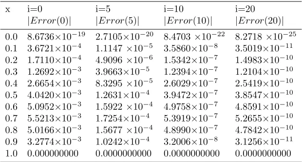
Table 4. Comparison of absolute errors for u(x,2) at m = 3 and T = 2 with different values ofifor Example 5.2 by modified method.
x i=0 i=5 i=10 i=20
|Error(0)| |Error(5)| |Error(10)| |Error(20)|
0.0 8.6736×10⁻¹⁹ 2.7105×10⁻²⁰ 8.4703×10⁻²² 8.2718×10⁻²⁵ 0.1 3.6721×10⁻⁴ 1.1147×10⁻⁵ 3.5860×10⁻⁸ 3.5019×10⁻¹¹ 0.2 1.7110×10⁻⁴ 4.9096×10⁻⁶ 1.5342×10⁻⁷ 1.4983×10⁻¹⁰ 0.3 1.2692×10⁻³ 3.9663×10⁻⁵ 1.2394×10⁻⁷ 1.2104×10⁻¹⁰ 0.4 2.6654×10⁻³ 8.3295×10⁻⁵ 2.6029×10⁻⁷ 2.5419×10⁻¹⁰ 0.5 4.0420×10⁻³ 1.2631×10⁻⁴ 3.9472×10⁻⁷ 3.8547×10⁻¹⁰ 0.6 5.0952×10⁻³ 1.5922×10⁻⁴ 4.9758×10⁻⁷ 4.8591×10⁻¹⁰ 0.7 5.5213×10⁻³ 1.7254×10⁻⁴ 5.3919×10⁻⁷ 5.2655×10⁻¹⁰ 0.8 5.0166×10⁻³ 1.5677×10⁻⁴ 4.8990×10⁻⁷ 4.7842×10⁻¹⁰ 0.9 3.2774×10⁻³ 1.0242×10⁻⁴ 3.2006×10⁻⁸ 3.1256×10⁻¹¹ 1.0 0.000000000 0.0000000000 0.0000000000 0.0000000000
Example 5.3. Consider the following space fractional diffusion equation [14]
∂u(x, t)
∂t =q(x)
∂αu(x, t)
∂xα +s(x, t), 0< x <1 (5.10)
with initial conditionu(x,0) =x4, and boundary conditions
u(0, t) = 0, u(1, t) =e−t,
where the function s(x, t) =−2e−tx4 is a source term, and q(x) = 1
24Γ(5−α). The exact solution to this equation ise−tx4.
Table 5. Comparison of absolute errors for u(x,2) at m = 3 and T = 2 with different values ofifor Example 5.2 by modified method.
x i=25 i=30 i=35 i=45
|Error(25)| |Error(30)| |Error(35)| |Error(45)|
0.0 2.5849×10⁻²⁶ 0.0000000000 2.5243×10⁻²⁹ 2.4651×10⁻³² 0.1 1.0904×10⁻¹¹ 3.4199×10⁻¹² 1.0687×10⁻¹⁴ 9.9746×10⁻¹⁸ 0.2 4.6822×10⁻¹² 1.4632×10⁻¹² 4.5727×10⁻¹⁵ 5.2041×10⁻¹⁸ 0.3 3.7826×10⁻¹¹ 1.1820×10⁻¹² 3.6939×10⁻¹⁵ 3.6429×10⁻¹⁷ 0.4 7.9436×10⁻¹¹ 2.4823×10⁻¹² 7.7573×10⁻¹⁴ 7.9797×10⁻¹⁷ 0.5 1.2046×10⁻¹⁰ 3.7644×10⁻¹² 1.1764×10⁻¹² 1.1796×10⁻¹⁶ 0.6 1.5185×10⁻¹⁰ 4.7452×10⁻¹² 1.4823×10⁻¹⁴ 1.5265×10⁻¹⁶ 0.7 1.6454×10⁻¹⁰ 5.1421×10⁻¹² 1.6069×10⁻¹⁴ 1.6653×10⁻¹⁶ 0.8 1.4995×10⁻¹⁰ 4.6721×10⁻¹² 1.4600×10⁻¹⁴ 1.5265×10⁻¹⁶ 0.9 9.7975×10⁻¹¹ 3.0523×10⁻¹² 9.5382×10⁻¹⁴ 1.1102×10⁻¹⁶ 1.0 0.0000000000 2.7755×10⁻¹⁷ 0.0000000000 2.7755×10⁻¹⁷
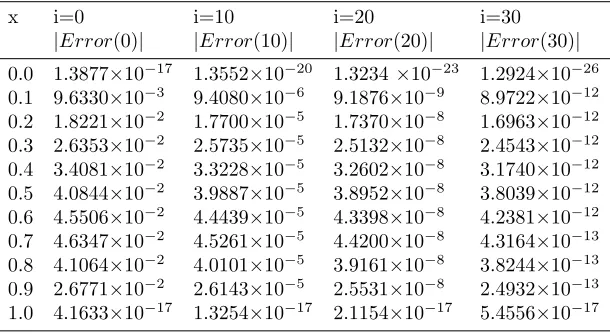
Table 6. Comparison of absolute errors for u(x,1) at m = 4 and T = 1 with different values ofifor Example 5.3 by modified method.
x i=0 i=10 i=20 i=30
|Error(0)| |Error(10)| |Error(20)| |Error(30)|
0.0 1.3877×10⁻¹⁷ 1.3552×10⁻²⁰ 1.3234×10⁻²³ 1.2924×10⁻²⁶ 0.1 9.6330×10⁻³ 9.4080×10⁻⁶ 9.1876×10⁻⁹ 8.9722×10⁻¹² 0.2 1.8221×10⁻² 1.7700×10⁻⁵ 1.7370×10⁻⁸ 1.6963×10⁻¹² 0.3 2.6353×10⁻² 2.5735×10⁻⁵ 2.5132×10⁻⁸ 2.4543×10⁻¹² 0.4 3.4081×10⁻² 3.3228×10⁻⁵ 3.2602×10⁻⁸ 3.1740×10⁻¹² 0.5 4.0844×10⁻² 3.9887×10⁻⁵ 3.8952×10⁻⁸ 3.8039×10⁻¹² 0.6 4.5506×10⁻² 4.4439×10⁻⁵ 4.3398×10⁻⁸ 4.2381×10⁻¹² 0.7 4.6347×10⁻² 4.5261×10⁻⁵ 4.4200×10⁻⁸ 4.3164×10⁻¹³ 0.8 4.1064×10⁻² 4.0101×10⁻⁵ 3.9161×10⁻⁸ 3.8244×10⁻¹³ 0.9 2.6771×10⁻² 2.6143×10⁻⁵ 2.5531×10⁻⁸ 2.4932×10⁻¹³ 1.0 4.1633×10⁻¹⁷ 1.3254×10⁻¹⁷ 2.1154×10⁻¹⁷ 5.4556×10⁻¹⁷
follows:
u4(x,1) = 4 X
i=0
λi(t)Pi∗(x) = 1.3877×10⁻¹⁷+ 0.1051x−0.11004x2+ (5.11)
0.2478x3+ 0.1249x4.
Table 7. Comparison of absolute errors for u(x,1) at m = 4 and T = 1 with different values ofifor Example 5.3 by modified method.
x i=50 i=60 i=70 i=80
|Error(50)| |Error(60)| |Error(70)| |Error(80)|
0.0 1.2326×10⁻³² 1.2037×10⁻²⁵ 1.1754×10⁻²⁸ 1.1479×10−41 0.1 8.5545×10⁻¹⁸ 8.1621×10⁻²¹ 7.9708×10⁻²⁴ 7.7840×10⁻²⁷ 0.2 1.6170×10⁻¹⁷ 1.4415×10⁻²⁰ 1.4077×10⁻²³ 1.3747×10⁻²⁶ 0.3 2.3546×10⁻¹⁷ 1.8759×10⁻²⁰ 1.8319×10⁻²³ 1.7890×10⁻²⁶ 0.4 3.0377×10⁻¹⁷ 2.1195×10⁻²⁰ 2.0698×10⁻²³ 2.0213×10⁻²⁶ 0.5 3.6120×10⁻¹⁷ 2.1721×10⁻²⁰ 2.1212×10⁻²³ 2.0715×10⁻²⁶ 0.6 4.1643×10⁻¹⁷ 2.0339×10⁻²⁰ 1.9862×10⁻²³ 1.9396×10⁻²⁶ 0.7 3.1334×10⁻¹⁷ 1.7047×10⁻²⁰ 1.6648×10⁻²³ 1.6257×10⁻²⁶ 0.8 3.9887×10⁻¹⁷ 1.1847×10⁻²⁰ 1.1569×10⁻²³ 1.1298×10⁻²⁶ 0.9 3.2607×10⁻¹⁷ 4.7381×10⁻²¹ 4.6271×10⁻²² 4.5187×10⁻²⁷ 1.0 4.3826×10⁻¹⁸ 4.2798×10⁻²¹ 4.1795×10⁻²⁴ 4.0816×10⁻²⁷
Example 5.4. In this example, we consider the following space fractional diffusion equation [13]
∂u(x, t)
∂t =q(x)
∂1.5u(x, t)
∂x1.5 +s(x, t), 0< x <1, (5.12)
with the initial condition
u(x,0) = (x2+ 1) sin(1),
and boundary conditions
u(0, t) sin(t+ 1), u(1, t) = 2 sin(t+ 1), f or t >0,
the source functions(x, t) = (x2+ 1) cos(t+ 1)−2xsin(t+ 1),andq(x) = Γ(1.5)x0.5.
The exact solution of this problem isu(x, t) = (x2+ 1) sin(t+ 1).
By using the proposed method [10], the polynomial approximation is as follows:
u2(x,1) = 2 X
i=0
λi(t)Pi∗(x) = 0.9092 + 0.2276x+ 0.6816x
2. (5.13)
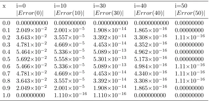
In Table 8 we have reported the comparison between exact and approximate so-lution for m = 2 and ∆t = 0.001 and final time T = 1 with different values of
i.
6. Conclusion
Table 8. Comparison of absolute errors for u(x,1) at m = 2 and T = 1 with different values ofifor Example 5.4 by modified method.
x i=0 i=10 i=30 i=40 i=50
|Error(0)| |Error(10)| |Error(30)| |Error(40)| |Error(50)|
0.0 0.000000000 0.000000000 0.0000000000 0.0000000000 0.00000000 0.1 2.049×10⁻² 2.001×10⁻⁵ 1.908×10⁻¹⁴ 1.865×10⁻¹⁶ 0.00000000 0.2 3.643×10⁻² 3.557×10⁻⁵ 3.392×10⁻¹⁴ 3.308×10⁻¹⁶ 1.11×10⁻¹⁶ 0.3 4.781×10⁻² 4.669×10⁻⁵ 4.453×10⁻¹⁴ 4.352×10⁻¹⁶ 0.00000000 0.4 5.464×10⁻² 5.336×10⁻⁵ 5.089×10⁻¹³ 4.962×10⁻¹⁶ 0.00000000 0.5 5.692×10⁻² 5.558×10⁻⁵ 5.301×10⁻¹³ 5.173×10⁻¹⁶ 0.00000000 0.6 5.466×10⁻² 5.336×10⁻⁵ 5.089×10⁻¹³ 4.984×10⁻¹⁶ 1.11×10⁻¹⁶ 0.7 4.781×10⁻² 4.669×10⁻⁵ 4.453×10⁻¹⁴ 4.340×10⁻¹⁶ 1.11×10⁻¹⁶ 0.8 3.643×10⁻² 3.557×10⁻⁵ 3.392×10⁻¹⁴ 3.308×10⁻¹⁶ 1.11×10⁻¹⁶ 0.9 2.049×10⁻² 2.001×10⁻⁵ 1.908×10⁻¹⁴ 1.865×10⁻¹⁶ 0.00000000 1.0 0.00000000 1.110×10⁻¹⁶ 1.110×10⁻¹⁶ 0.000000000 0.00000000
Caputo sense. Comparison between our proposed method with exact solution, shows that this method is effectively accurate and evidently the error gets smaller as the calculation stages go ahead.
Acknowledgements
It should be mentioned that the above article has been derived from the ph. d thesis of the H. Jaleb, at the Islamic Azad University Central Tehran Branch.
References
[1] L. Bagley and P. J. Torvik,On the appearance of the fractional derivative in the behavior of real materials, J. Appl. Mech.,51(1984), 294-298.
[2] C. Canuto, A. Quarteroni, M. Y. Hussaini, and T. A. Zang,Spectral methods fundamentals in single domains, Springer-Verlag Berlin Heidelberg, Printed in Germany, 2006.
[3] R. Darzi, B. Mohammadzade, S. Musavi, and R. Behshti,Sumudu transform method for solving fractional differential equations and fractional diffusion-wave equation, J. Math. Comput.Sci. (TJMCS),6(2013), 79–84.
[4] S. Das,Fractional calculus for system identification and controls, Springer, New york, 2008. [5] G. J. Fix, J.P. Roop,Least squares finite element solution of the fractional order two-point
boundary value problem,Comput.Math.Apple,48(2004), 1017-1033.
[6] I. Hashim, O. Abdulaziz, and S. Momani,Homotopy analysis method for fractional IVPs, Com-mun. Nonlinear Sci. Numer. Simul.,14(2009), 674-684.
[7] M. Inc,The approximate and exact solutions of the space-and time-fractional Burger’s equations with initial conditions by varational iteration method, Math. Anal. Apple,345(2008), 476–484. [8] H. Jafari and V. Daftardar-Gejji, Solving linear and nonlinear fractional diffusion and wave
equations by ADM, Appl. Math. and Comput,180(2006), 488-497.
[9] M. J. Kimeu,Fractional calculus: definitions and applications, 2009. Thesis (Ph. D.)–University of Western Kentucky - Kentucky
[11] M. M. Khader, N. H. Swetlam, and A. M. S. Mahdy,The Chebyshev collection method for solv-ing fractional order Klein-Gordon equation, WSEAS Transactions on Mathematics,13(2014), 2224–2880 .
[12] M. M. Khader, N. H. Sweilam, and A. M. S. Mahdy,An Efficient numerical method for solving the fractional diffusion equation, Journal of Applied Mathematics and Bio Informatics,1(2011), 1–12.
[13] F. Liu, V. Anh, and I. Turner,Numerical solution of the space fractional Fokker-Plank equation ,J.Comput.Apple.Math,166(2004), 209-219.
[14] F. Liu, V. Anh, I. Turner, and P. Zhuang, Time fractional advection dispersion equation , Journal of Applied Mathematics and Computation,13(2003), 233-245.
[15] K. S. Miller and B. Ross,An introduction to the fractional calculus and fractional differential equations, John Wiley, New York, 1993.
[16] M. M. Meerschaert and C. Tadjeran,Finite difference approximations for fractional advection-dispersion flow equations, J. Comput. Appel. Math.,172(2008), 65–77.
[17] M. M. Meerschaert and C. Tadjeran, Finite difference approximations for two-sided space-fractional partial differential equations, Appel. Numer. Math.,56(2006), 80–90.
[18] A. Neamaty, B. Agheli, and R. Darzi,Solving fractional partial differential equation by using wavelet operational method, J. Math. Comput. Sci. (TJMCS),7(2013), 230–240.
[19] K. B. Oldham and J. Spanier,The fractional calculus, Academic Press, New York and London, 1974.
[20] I. Podlubny,Fractional differential equations, Academic Press, New York, 1999.
[21] E. A. Rawashdeh,Numerical solution of fractional integro-differential equations by collocation method, Apple. Math. Comput.,176(2006), 1–6.
[22] S. G. Samko, A. A. Kilbas, and O. I. Marichev,Fractional integrals and derivatives: theory and applications, Gordon and Breach Science Publishers, USA, 1993.
[23] N. H. Sweilam, M. M. Khader, and R. F. AL-Bar,Numerical studies for a multi-order fractional differential equation,Physics Letters A,371(2007), 26–33.
[24] A. Saadatmandi and M. Dehghan,A Tau approach for solution of the space fractional diffusion equation, Comput. Math. Apple,62(2011), 1135–1142.