A Methodology for Quantifying the Kinematic Position
Errors due to Manufacturing and Assembly Tolerances
Flores, P.
Paulo Flores*
CT2M/ Department of Mechanical Engineering, University of Minho, Portugal
A systematic and general methodology for kinematic position errors analysis of multibody systems is investigated throughout this work, taking into account the influence of the manufacturing and assemble tolerances on the performance of planar mechanisms. The generalized Cartesian coordinates are used to mathematically formulate kinematic constraints and equations of motion of the multibody systems. Thus, the systems are defined by a set of generalized coordinates, which represents the instantaneous positions of all bodies, together with a set of generalized dimensional parameters that defines the functional dimensions of the system. These generalized dimensional parameters take into account the tolerances associated with the lengths, fixed angles, diameters and distance between centers, among others. This paper highlights the relation among kinematic constraints, dimensional parameters and output kinematic parameters. Based on the theory of dimensional tolerances, the variation of the geometrical dimensions is regarded as a tolerance grade with an interval associated with each dimension and, consequently, a kinematic amplitude variation for the bodies’ position. The methodology presented is implemented in a computational code developed for kinematic analysis of multibody systems, capable of automatically generating and solving the equations of motion for general multibody systems. Finally, a slider-crank mechanism is used as a numerical example to demonstrate the accuracy of the presented methodology, as well as to discuss the main assumptions and procedures adopted in this work.
©2011 Journal of Mechanical Engineering. All rights reserved.
Keywords: positional error, manufacturing tolerances, assembly systems, planar mechanisms
0 INTRODUCTION
It is well known that the tolerances play a key role in the modern design process by introducing quality improvements and limiting manufacturing costs. According to standard ANSI Y14.5M-1994, tolerances are used to define the allowable limits of geometric variation that are inherent in manufacturing and assemble processes [1]. Thus, the assignment of geometric tolerances is always a trade-off between two distinct situations: (i) a part with tight tolerances is good for assembly, but the cost to manufacture the part is increased; (ii) alternatively, loose tolerance in one part may make the whole assemble infeasible. The tolerance analysis deals with the study of the aggregate behaviors of given individual tolerances [2] and [3].
Over the last few decades a number of research papers have been published on the influence of the tolerance and clearance on the kinematic performance of multibody systems [4] to [14]. However, most of these research works
approach required that constraint equations to be known and independent. Flores et al. [11] and [12] studied the influence of clearance in joints on the kinematic and dynamic performance of multibody systems. These works are valid for both planar and spatial systems and for dry and lubricated joints; however, they do not account for tolerance effects. Dong and Ye [13] modeled and studied a reheat-stop mechanism considering the effects of tolerance, misalignment and thermal action. A good survey on the research work developed in the field of tolerance analysis of kinematic mechanism is provided by Chase and Parkinson [14].
By and large, there are two main approaches to study the effect of the manufacturing tolerances on the kinematic position errors, namely, the deterministic and probabilistic methods. The deterministic method involves fixed values or constraints that are used to find an exact solution. These methods are used mostly when tolerances are known and the worst position error is to be determined. In contrast, the probabilistic or statistical methods deal with random variables that result in a probabilistic response. The statistical approaches are utilized when dimensions have some type of random distribution and the probability of being within a given tolerance band is to be evaluated.
Chase and Greenwood [15] introduced a statistical model to sum tolerances of characteristics affected by variability with mean shift. This model weights the values of tolerances sum between two extremes cases: (i) the worst case and (ii) the root sum square case. The worst case model assumes that all the component dimensions occur, in each assembly, at their extreme and worst limit simultaneously. The root sum square method considers that the component dimensions occur statistically having a Gaussian distribution. From statistical point of view the worst model is the most pessimistic evaluation of the sum variability, meanwhile the root sum square is the more optimistic evaluation of the sum variability.
In general, the manufacturing cost increases geometrically for uniform incremental tightening of tolerances [16]. The cost is also related to the characteristics of manufacturing processes used, and the degree of maturity of the workers. The
allocated tolerances should be as large as possible for the sake of economy and ease of manufacture. However, large tolerances usually increase mechanical errors. Thus, designers should allocate tolerances to minimize the manufacturing cost while keeping mechanical errors below a certain specific limit [17].
The main purpose of this research work is to present a general and systematic approach to quantify the kinematic position errors due to manufacturing and assemble tolerances. Based on the worst case the deterministic method is utilized. The kinematic constraints and equations of motion of the multibody systems are formulated under the framework of multibody systems methodologies. The system is defined by a set of generalized coordinates, which represents the instantaneous positions of all bodies, together with a set of generalized dimensional parameters that defines the functional dimensions of the system. The generalized dimensional parameters take into account the tolerances associated with the lengths. The relation between the kinematic constraints, dimensional parameters and output kinematic parameters is demonstrated. Finally, the proposed methodology is applied to an elementary planar multibody system in order to demonstrate its features.
1 KINEMATIC ANALYSIS
The kinematic analysis is the study of the motion of a system, independently of the forces that produce it. Since in the kinematic analysis the forces are not considered, the motion of the system is specified by driving elements that govern the system motion during the analysis, while the position, velocity and acceleration of the remaining elements are defined by kinematic constraint equations that describe the system topology. It is clear that in the kinematic analysis, the number of driver constraints must be equal to the number of degrees of freedom of the multibody mechanical system. In short, the kinematic analysis is performed by solving a set of equations that result from the kinematic and driver constraints.
holonomic constraints Φ can be written in a compact form as [18] to [20],
Φ(q,t) = 0, (1) where q is the vector of generalized coordinates and t is the time variable, usually associated with the driving elements.
The velocities and accelerations of the system elements are evaluated through the velocity and acceleration constraint equations. Thus, the first time derivative with respect to time of Eq. (1) provides the velocity constraint equations:
ΦΦqq= − ≡ΦΦ υυt , (2) where Φq is the Jacobian matrix of the constraint
equations, that is, the matrix of the partial derivates, ∂Φ/∂q, q is the vector of generalized velocities and υ is the right hand side of velocity equations, which contains the partial derivates of Φ with respect to time, ∂Φ/∂t. It should be noticed that only rheonomic constraints, associated with driver equations, contribute with non-zero entries to the vector υ. Furthermore, it is assumed that this vector does not present any dependency on the vector of coordinates.
A second differentiation of Eq. (1) with respect to time leads to the acceleration constraint equations, obtained as:
Φ
Φqq= −(ΦΦqq q )q −2ΦΦqtq−ΦΦtt ≡γγ, (3) where q is the acceleration vector and γ is the right hand side of acceleration equations, i.e., the vector of quadratic velocity terms, which contains the terms that are only function of velocity, position and time. In the case of scleronomic constraints, that is, when Φ is not explicitly dependent on the time, the term Φt in Eq. (2) and the Φqt and Φtt
terms in Eq. (3) vanish.
The constraint equations represented by Eq. (1) are, in general, non-linear in terms of q and are usually solved by the Newton-Raphson method. Eqs. (2) and (3) are linear in terms of
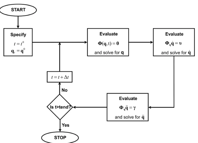
q and q, respectively, and can be solved by any usual method for linear equations’ systems. Thus, the kinematic analysis of a multibody system can be carried out by solving the set of Eqs. (1) to (3). The necessary steps to perform this analysis are sketched in Fig. 1, and described as,
(i) Specify the initial conditions for positions q0 and initialize the time counter t0.
(ii) Evaluate the position constraint Eq. (1) and solve it for positions, q.
(ii) Evaluate the velocity constraint Eq. (2) and solve it for velocities, q.
(iv) Evaluate the acceleration constraint Eq. (3) and solve it for accelerations, q.
(v) Increment the time. If the time is smaller than final time, go to step ii), otherwise stop the analysis.
2 MATHEMATICAL FORMULATION OF THE KINEMATIC POSITION ERRORS DUE TO
TOLERANCES
In order to evaluate, in a systemic and general way, the influence of the manufacturing and assemble tolerances on the kinematic position errors, special attention needs to be given to the mathematical formulation of the description of the systems’ configuration. Thus, according to the previous section, the equations of constraints can be written as:
Φ(q1, q2, ..., qn, d1, d2, ..., dm)=0 , (4) where q1, q2, ..., qn represent the generalized vector of coordinates that define the kinematic system’s configuration at any instant, and d1, d2, ..., dm are the generalized vectors of the dimensional parameters defining the functional dimensions of the system. It should be noted that Eq. (4) represents the kinematic system’s constraints, which can easily be written using, for instance, Cartesian coordinates. Furthermore, the number of generalized coordinates, n, and the number of generalized dimensional parameters, m, must be adequately selected bearing in mind the correct system’s description and system’s degrees of freedom.
The kinematic analysis of any multibody system implies the resolution of Eq. (4) for q1, q2, ..., qn and their derivatives, according to what was presented in the previous section. In this process, it is assumed that vectors d1, d2, ..., dm are constants, meaning that there is no variation of the dimensional parameters and, consequently, that they do not affect the global system’s performance. However, it is well known that this is not the case in practical engineering design and manufacturing processes.
Since, in general, multibody systems are conducted by driving elements, excluding these elements and considering that the kinematic constraints are independent, the Jacobian matrix can be written as follows:
ΦΦq ΦΦ q
=∂
∂ kl , (k = 1, …, n-dr; l = 1, …, n), (5) where indices k and l represent, respectively, the n-dr kinematic constraints and n Cartesian coordinates. The number of driving elements is represented by variable dr.
Considering all coordinates and dimensional parameters as global system’s variables, the variation of the constraint equation is expressed as:
∂
∂ + +
∂
∂ +
∂
∂ + +
∂
∂ =
Φ
Φk ΦΦk ΦΦ ΦΦ
n n
k k
m m
q1 q q q d d d d 0
1
1 1
δ ... δ δ ... δ ,. (6)
In a compact form, Eq. (6) is be written as:
∂
∂ +
∂
∂ =
= −
=
∑
ΦΦk∑
ΦΦi i i
n dr
k
j j j
m
q δq d δd 0
1 1
, (k = 1, …, n-dr) (7)
in which, δqi is the variation of the generalized system’s coordinates and δdj is the variation of the dimensional parameters. This last term represents the manufacturing tolerances of the corresponding functional dimensions, such as the lengths of the multibody system parts.
In a matrix form, Eq. (7) is expressed as:
Φ
Φqiδqi = −ΦΦdjδdj, (i = 1, …, n-dr, j = 1, …, m), (8)
where ΦΦqi is the Jacobian matrix and ΦΦdi represents the derivative of the constraint equations in relation to the dimensional parameters.
Since in the kinematic analysis of multibody systems the Jacobian matrix is known, as illustrated in the previous section, specifying the manufacturing tolerances, δdj , only the matrix
ΦΦdi needs to be evaluated in order to obtain the kinematic position errors of all system’s bodies, by solving Eq. (8). It should be noted, that with this approach very low computational effort is added to the standard kinematic analysis procedure. Moreover, it should be highlighted that Eq. (8) represents a linear system of equations that can easily be solved by employing any numerical method, such as the LU factorization procedure, available in the thematic literature [21] and [22].
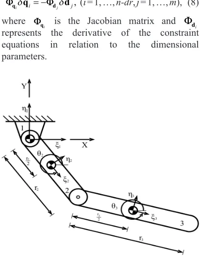
With the intent to illustrate the application of this approach, a double pendulum system demonstrative example follows. Fig. 2 shows the double pendulum, where the body numbers, local and global coordinate systems are illustrated. Since this simple multibody system has two ideal revolute joints, the corresponding constraint equations expressed in Cartesian coordinates are written as:
Φ1 2 2 2
2 0
≡ − −x r cosθ = , (9)
Φ2 2 2
2
2 0
≡ − −y r sinθ = , (10)
Φ3 2 2
2 3 3 3
2 2 0
≡x +r cosθ − −x r cosθ = , (11)
Φ4≡y2+r22sinθ2−y3−r23sinθ3=0, (12)
where x2, y2, θ2, x3, y3 and θ3 are the global system coordinates and r2 and r3 are the selected dimensional tolerance parameters. The input parameters corresponding to the driving elements are the angles θ2 and θ3, being x2, y2, x3, and y3 the output parameters. The differentiation of the constraints’ Eqs. (9) to (12) yields the variation of the constraints as follows:
δΦ1 δ 2 θ2δ
2
2 0
≡ − x −cos r = , (13)
δΦ2 δ 2 θ2δ
2
2 0
≡ − y −sin r = , (14)
δΦ3 δ 2 θ2δ δ θ δ
2 3 3 3
2 2 0
≡ x +cos r − x −cos r = , (15)
δΦ4 δ 2 θ2δ δ θ δ
2 3 3 3
2 2 0
≡ y +sin r − y −sin r = . (16)
Rearranging Eqs. (13) to (16) results:
-1 0 0 0 0 1 0 0 1 0 1 0 0 1 0 1
2 2 3 3 δ δ δ δ x y x y == cos sin cos cos sin sin θ θ θ θ θ θ δ 2 2 2 3 2 3 2 2 2 2 2 2 0 0 -r22 3 δr , (17)
which represents a linear system of equations that can be solved for the unknowns δx2, δy2, δx3 and δy3, since the values of the variables θ2 and θ3 are specified as inputs and δr2 and δr3 represent the tolerance amplitude for the double pendulum arm lengths r2 and r3.
In a compact form Eq. (17) is be written as: Φqδq = –Φdδd (18)
Again, from Eq. (18) great simplicity and generality of the proposed methodology for the study of kinematic position errors due to manufacturing tolerances is evident. In Eq. (18) the term Φq, which corresponds to the partial
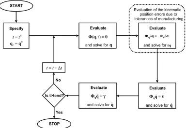
derivatives of the constraint equations with respect to the dimensional parameters, represents the quantitative influence of the individual variation of the selected dimensional tolerance parameters on the kinematic accuracy of the output parameters. Fig. 3 shows the flowchart of the computational procedure to perform kinematic analysis of a multibody system, in which the kinematic position errors owing to tolerances are evaluated.
procedure. Obviously, it is possible to complete the standard kinematic analysis, and then go back at each step of time simulated and evaluate the position error analysis be solving Eq. (18). However, this way requires to store the history response, being easier and computationally more efficient to perform the position error analysis at each step of the standard kinematic procedure. The problem of sensitivity analysis of mechanical systems has grasped the attention of several authors such as Arora and Haug [23], Lee et al. [24], Schulz and Brauchli [25], only to mention a few. Furthermore, the problem of optimization and parameter identification of multibody system models using gradient based optimization methods has been developed by Bock and his co-workers [26] and [27].
In order to quantify the kinematic accurate position of a multibody system link, it is first necessary to define the amount of tolerance allowed for each of the dimensional parameters considered. Thus, according to standard ISO 286-1, for common mechanical operating conditions the IT grades are usually in the range IT8 to IT11
[17]. For the manufacturing tolerances of the dimensional parameters of a multibody system, the bilateral tolerances specified in ISO 286-1 are commonly used. Hence, in Eq. (18), the variation of the functional parameters δd can be regarded as such tolerance fields. Therefore, it is possible to write the following relation:
δd = ±½T , (19) where T represents the total manufacturing tolerance range corresponding to the dimensional parameters.
3 MANUFACTURING AND ASSEMBLY TOLERANCE ANALYSIS
It is known that tolerances are used to define the allowable limits of geometric variations that are inherent in the manufacturing and assembly processes [1]. Broadly, there are two approaches to solve this problem; worst case assemblability and statistical assemblability. In the first case, it is assumed that all the component dimensions
occur, in each assembly, at their extreme and worst limit simultaneously. When this approach is employed, the designer desires to ensure that the components can always be assembled. This means that the probability of having a kinematic error exceeding the specific limits in a particular system is null. On the other hand, the statistical assemblability can be used to take advantage of statistical averaging over of components, allowing for the use of less restrictive tolerances in exchange for admitting the small probability of non-assembly. In general, the standard process is defined at the confidence level corresponding to ±3σ interval [28] and [29]. From the statistical point of view the worst case model is the most pessimistic, while the statistical assemblability is the most optimistic case. In practical situations it is expected that they fall between the worst and statistical models. These two approaches are discussed in detail in the following paragraphs. Using Eq. (18) as reference, the variation of the generalized system’s coordinates can be rewritten as:
δq = sδd , (20) where s represents the sensitive coefficients given by:
s= −ΦΦ Φq−1Φd. (21) Considering a system with m generalized dimensional parameters and that the maximum tolerance or error is specified, based on the worst scenario assemblability, it is possible to evaluate the maximum error of a general output coordinate as:
1
2 12
1 1
2 1 1 2 2
T s T
s T s T s T
maximum j j
j m
m m
≥ = =
=
(
+ + +)
=
∑
δq
... . (22)
The average tolerance can be determined by the following expression:
T
s T
m T
m
average
j j j
m
=
∑
= =1 2
1 maximum. (23)
In a similar way, the tolerance associated with any system component can be given by:
T T s m
i i
= maximum. (24)
It is worth noting that Tmaximum is a given quantity, allowing the evaluation of average
tolerance values, which ultimately can be used as a guiding reference to specify the manufacturing precision requirements of the system components by selecting the IT grades.
Tolerance is statistical in nature since the output of a random variable is, in general, normally or Gaussian distributed, with the level of confidence three-sigma considered. This means that only two or three cases in a thousand have the probability to be outside the ±3σ range. This confidence level of tolerance becomes an important design parameter to be evaluated and optimized. Thus, using the statistical approach, the root mean square considers that the component dimensions occur statistically having a Gaussian distribution and can be expressed by:
1
2 2 12
2
1
T sj Tj
j m
maximum≥ =
( )
=
∑
δq . (25)
In the statistical approach, the average tolerance can be determined by the following expression:
T T
m
average= maximum. (26)
In a similar way, the tolerance associated with any system component can be given by:
T T s m
i i
= maximum. (27)
In order to convert the tolerance value to the standard process-tolerance, the γ factor is introduced [3]:
γ σ =Tmaximum
2 . (28)
Solving Eq. (28) for σ yields:
σ γ =Tmaximum
2 . (29)
Consequently, the admissible tolerance of any component can be expressed by:
Tadmissible =6σ =3Tmaximumγ . (30)
p f e dt
100
1 2
22
= =
−
∫
( )γ / .
π γ γ
γ (31)
Table 1. Values of γ factor for different confidence levels
p = 99.7% f(γ) = 0.997 γ = 2.96 p = 99.0% f(γ) = 0.990 γ = 2.58 p = 97.0% f(γ) = 0.970 γ = 2.17 p = 95.0% f(γ) = 0.950 γ = 1.96
4 EXAMPLE OF APPLICATION: SLIDER-CRANK MECHANISM
An elementary slider-crank mechanism is used here to show the influence of manufacturing tolerances on kinematic performance. Fig. 4 shows the configuration of the mechanism, comprising four rigid bodies that represent the crank, connecting rod, slider and ground, three revolute joints and one ideal translational joint. The inertia properties and length characteristics of each body, as well as the associated tolerance according to ISO 286-1 standard are given in Table 2. In the present example the tolerance grade IT 10 was selected establishing the number of generalized dimensional parameters equal to two (m = 2), which are related to the lengths of the crank (r2) and connecting rod (r3).
Fig. 4. Schematic representation of the slider-crank mechanism
Table 2. Geometric properties of the slider-crank mechanism
Body
Nr. Description Length [m] Tolerance range [mm]
1 Ground -
-2 Crank 0.050 ± 50
3 Connecting rod 0.120 ± 70
4 Slider -
-In the kinematic simulation, the crank is the driving element and rotates at a constant angular
velocity of 500 rpm clockwise. The initial system configuration corresponds to the top dead point. In the numerical simulation, r2 and r3 were selected as dimensional tolerance parameters, being δx4 and δθ3 the output parameters. Thus, applying the methodologies presented in the previous sections, Figs. 5 and 6 show, respectively, the maximum absolute errors on the linear slider position and the angular position of the connecting rod, when the worst case approach is considered. These maximum position errors were evaluated at 25 crank angular positions. By observing the obtained global results it can be concluded that the maximum position errors vary during the computational simulation of the slider crank mechanism.
Fig. 5. Maximum linear position error of the slider evaluated over a complete crank cycle
Fig. 6. Maximum angular position error of the connecting rod evaluated over a full crank cycle
´ x cos¸ sin¸ tan¸ ´ r cos¸ sin¸ tan¸ ´ r
4 2 2 3 2
3 3 3 3
= ±
(
+)
++
(
+)
, (32)or in another form:
δx4= ±
(
s T s T112 1+ 212 2)
, (33)where the manufacturing tolerances on dimensions r2 and r3 are represented by T1 and T2, and the sensitive coefficients s1 and s2 can be written as follows:
s1 = cosθ2 + sinθ2 tanθ3 , (34) s2 = cosθ3 + sinθ3 tanθ3 , (35) From the analysis of Fig. 5, it can be observed that the most critical situation occurs when the crank and the connecting rod are collinear, that is, when θ2 = 0 or 180º and θ3 = 180º. In these circumstances, the sensitive coefficients s1 and s2 are equal to 1. When the worst case is considered, the maximum tolerance can be calculated using Eq. (22) yielding:
Tmaximum= ±
(
s T s T+)
== ± ×
(
+ ×)
= ±112 1 212 2
1 50 1 70 120µm.
It is obvious that this value is relatively high from a practical engineers view point. On the other hand, when the statistical model is considered, the maximum tolerance is determined using Eq. (25), that is:
Tmaximum= ±
(
s T)
+(
s T)
== ±
(
×)
+ ×(
)
= ±112 1 2
212 2 2
2 2
1 50 1 70 86µm. This value is still high for practical purposes. Therefore, considering, for example that the maximum admissible tolerance is equal to ±55 μm, then the γ factor can be evaluated using Eq. (30):
Tadmissible= T ⇒ =
× =
3 3 55
86 1 92
maximum
γ γ . .
This value corresponds to a level of confidence less than 95%, which is far too high. With the intent to increase the confidence level, the sensitive coefficients associated with the tolerance dimensions should have larger values. This desideratum can be achieved by reducing the tolerance grade IT, for instance from 10 to 9 [17]. Consequently, according to ISO 286-1 standard the corresponding tolerance ranges of grade IT 9
for crank and connecting rod lengths are ±31 μm and ±44 μm. Thus, the maximum tolerance is now:
Tmaximum= ±
(
1 31×)
+ ×(
1 44)
= ±542 2
µm . Hence, the γ factor is evaluated as:
γ =3 55× =
54 3 06. .
The corresponding confidence level is over 99.7%, which can be considered to be clearly satisfactory.
5 CONCLUDING REMARKS
In this paper, a general and systematic methodology for kinematic positional error analysis of multibody systems was investigated, taking into account the influence of the manufacturing and assembly tolerances on the performance of planar mechanisms. In the process, the main aspects for kinematic analysis of multibody systems were revised. Based on the theory of dimensional tolerances, the variation of the geometrical dimensions is regarded as a tolerance grade with an interval associated with each dimension and, consequently, a kinematic amplitude variation for the positions. The presented deterministic method evaluates the relation between variations in the dimensional parameters and variation in the generalized coordinates. The statistical approach based on the confidence level three-sigma was also studied. The methodologies proposed have been exemplified through the application of kinematics to a slider-crank mechanism. The simplicity and generality of the proposed methodology for the study of kinematic position errors due to manufacturing tolerances was thus demonstrated. It should be highlighted that in this paper, only dimensional parameters such as length of links have been addressed. However, other parameters can be integrated in the general methodology presented throughout this work, namely those related to roundness of circular surfaces and clearances in joints.
6 ACKNOWLEDGMENTS
7 REFERENCES
[1] ANSY, Y14.5M-1994. (1994). Dimensional and Tolerancing, ASME, New York.
[2] Lee, W.J., Woo, T.C. (1990). Tolerances: Their Analysis and Synthesis. Journal of Engineering for Industry, vol. 112, p. 113-121.
[3] Di Stefano, P. (2006). Tolerances analysis and cost evaluation for product life cycle. International Journal of Production Research, vol. 44, no. 10, p. 1943-1961.
[4] Garrett, R.E., Hall, A.S. (1969). Effect of Tolerance and Clearance in Linkage Design. Journal of Engineering for Industry, vol. 91, p. 198-202.
[5] Dhande, S.G., Chakraborty, J. (1973). Analysis and Synthesis of Mechanical Error in Linkages – A Stochastic Approach. Journal of Engineering for Industry, vol. 95, p. 672-676.
[6] Hummel, S.R., Chassapis, C. (2000). Configuration design and optimization of universal joints with manufacturing tolerances. Mechanism and Machine Theory, vol. 35, p. 463-476.
[7] Shi, Z. (1997). Synthesis of mechanical error in spatial linkages based on reliability concept. Mechanism and Machine Theory, vol. 32, no. 2, p. 255-259.
[8] Choi, J.H., Lee, S.J., Choi, D.H. (1998). Tolerance Optimization for Mechanisms with Lubricated Joints. Multibody System Dynamics, vol. 2, p. 145-168.
[9] Wittwer, J.W., Chase, K.W., Howell, L.L. (2004). The direct linearization method applied to position error in kinematic linkages. Mechanism and Machine Theory, vol. 39, p. 681-693.
[10] Fogarasy, A.A., Smith, M.R. (1998). The influence of manufacturing tolerances on the kinematic performance of mechanisms. Journal of Mechanical Engineering Science, vol. 212, p. 35-47.
[11] Tian, Q., Zhang, Y., Chen, L., Flores, P. (2009). Dynamics of spatial flexible multibody systems with clearance and lubricated spherical joints. Computers and Structures, vol. 87, p. 913-929.
[12] Flores, P., Ambrósio, J., Claro, J.C.P., Lankarani, H.M. (2007). Dynamic behaviour of planar rigid multibody systems including revolute joints with clearance. Journal of Multi-body Dynamics, vol. 221, p. 161-174. [13] Dong, X., Ye, J. (2009). Performance Analysis
of the Reheat-Stop-Valve Mechanism under Dimensional Tolerance, Misalignment and Thermal Impact. Strojniški vestnik - Journal of Mechanical Engineering, vol. 55, no. 9, p. 507-520.
[14] Chase, K.W., Parkinson, A.R. (1991). A survey of research in the application of tolerance analysis to the design of mechanical assemblies. Research in Engineering Design, vol. 3, p. 23-37.
[15] Chase, K.W., Greenwood, W.H. (1988). Design issues in mechanical tolerance analysis. Manuf. Rev., vol. 1, no. 1, p. 50-59. [16] Drozda, T.J., Wick, C. (1983). Tool and
Manufacturing Engineers Handbook, Vol. I, Machining. 4th ed., SME, New York.
[17] ISO 286-1. (1988). ISO system of limits and fits – Parts 1: Base of tolerances, deviations and fits.
[18] Nikravesh, P.E. (1988). Computer Aided Analysis of Mechanical Systems. Prentice Hall, Englewood Cliffs, New Jersey.
[19] Shabana, A.A. (1989). Dynamics of Multibody Systems. John Wiley and Sons, New York. [20] Haug, E.J. (1989). Computer-Aided
Kinematics and Dynamics of Mechanical Systems - Volume I: Basic Methods, Allyn and Bacon, Boston, Massachusetts.
[21] Atkinson, K.E. (1989). An Introduction to Numerical Analysis, 2nd ed. John Wiley & Sons, New York.
[22] Amirouche, F.M.L. (1992). Computational Methods for Multibody Dynamics. Prentice Hall, Englewood Cliffs, New Jersey.
[23] Arora, J.S., Haug, E.J. (1979). Methods of design sensitivity analysis in structural optimization. AIAA Journal, vol. 17, no. 9, p. 970-974.
[25] Schulz, M., Brauchli, H. (2000). Two methods of sensitivity analysis for multibody systems with collisions. Mechanism and Machine Theory, vol. 35, no. 10, p. 1345-1365.
[26] Körkel, S., Kostina, E., Bock, H., Schlöder, J. (2007). Numerical methods for optimal control problems in design of robust optimal experiments for nonlinear dynamic processes. Optimization Methods and Software, vol. 19, p. 327-338.
[27] Diehl, M., Bock, H.G., Kostina, E. (2006). An approximation technique for robust nonlinear optimization. Mathematical Programming:
Series A and B Archive, vol. 107, no. 1, p. 213-230.
[28] Ang, A.H.S., Tang, W.H. (1984). Probability concepts in engineering planning and design. Vol. I - Basic principles. John Wiley & Sons, New York.
[29] Ang, A.H.S., Tang, W.H. (1984). Probability concepts in engineering planning and design. Vol. II - Decision, risk, and reliability. John Wiley & Sons, New York.