DEMOGRAPHIC RESEARCH
VOLUME 28, ARTICLE 43, PAGES 1263-1302
PUBLISHED 21 JUNE 2013
http://www.demographic-research.org/Volumes/Vol28/43/ DOI: 10.4054/DemRes.2013.28.43
Research Article
Probabilistic household forecasts
based on register data - the case of
Denmark and Finland
Solveig Glestad Christiansen
Nico Keilman
© 2013 Solveig Glestad Christiansen & Nico Keilman.
This open-access work is published under the terms of the Creative Commons Attribution NonCommercial License 2.0 Germany, which permits use, reproduction & distribution in any medium for non-commercial purposes, provided the original author(s) and source are given credit.
1 Introduction 1264 2 Overview of earlier work 1265
3 Methods 1269
3.1 Brief overview of our approach 1269 3.2 Deterministic household forecast 1269 3.3 Stochastic population forecast 1272 3.4 Analysis of time series data 1273 3.5 Simulation of household shares 1276
4 Data and assumptions 1278
5 Results 1286
5.1 Main outcomes 1286
5.2 Changing rates 1295
5.3 RWD extrapolations 1295
6 Conclusion 1295
7 Acknowledgements 1298
Probabilistic household forecasts based on register data - the case of
Denmark and Finland
Solveig Glestad Christiansen1 Nico Keilman2
Abstract
BACKGROUND
Household forecasts are important for public planning and for predicting consumer demand.
OBJECTIVE
The purpose of this paper is to compute probabilistic household forecasts for Finland and Denmark, taking advantage of unique housing register data covering the whole populations dating back to the 1980s. A major advantage is that we do not have to rely on small population samples, and we can get quite reliable estimates even for infrequent transitions. A further merit is having time series containing the population in different household positions (dependent child, living with a spouse, living in a consensual union, living alone, lone parent, living in other private household and institutional households) by age and sex.
METHODS
These series enable us to estimate the uncertainty in the future distribution of the population across household positions. Combining these uncertainty parameters with expected shares computed in a deterministic household forecast, we simulate 3000 sample paths for the household shares for each age and sex. These paths are then combined with 3000 simulations from a stochastic population forecast covering the same period to obtain the predicted number of households and persons in each household position by age and sex.
RESULTS
According to our forecasts, we expect a strong growth in the number of private households during a 30-year period, of 27% in Finland and 13% in Denmark. The
1 Corresponding author. Department of Economics, University of Oslo, P.O. Box 1095, 0317 Oslo.
E-mail: [email protected].
number of households consisting of a married couple or a person who lives alone are the most certain, and single parents and other private households are the most uncertain.
1. Introduction
Our aim is to compute probabilistic household forecasts for Denmark and Finland, using register data. Household forecasts are useful for planning housing supply, energy use, and the demand for consumer durables (e.g. King 1999; Muller, Gnanasekaran, and Knapp 1999; O’Neill and Chen 2002). For the elderly, the household position also has an effect on their demand for places in nursing homes (e.g. Lakdawalla and Philipson 1999; Lakdawalla et al. 2003; Grundy and Jital 2007).
Traditionally, household forecasts have been computed by models that, roughly speaking, can be divided in two groups: household headship rate models, and household transition models (Van Imhoff et al. 1995). Compared to headship rate models, which are static in nature, transition models have the advantage that they explicitly describe the dynamics of the household composition of the population.
Both types of models are widely used for computing deterministic forecasts. A projection of the number of households of a certain type in a given year in the future is computed as one number (or just a few numbers: see section 2). Such a deterministic forecast, however, does not give an accurate view of forecast uncertainty. The future is inherently uncertain, and hence probabilistic methods have to be used. Alho and Keilman (2010) have recently developed a method for computing probabilistic household forecasts. They applied their method to Norwegian data. One important drawback of their application is that the uncertainty assessments were based on limited data, and simplifying assumptions had to be made (see section 2).
The purpose of this paper is to improve on the approach of Alho and Keilman by taking advantage of high quality data from the population registers and housing registers of Denmark and Finland. Both countries have register data covering the whole populations dating back to the 1980s. The registers contain information about persons in every dwelling, including all flats in apartment blocks, each having its own unique address (Lind 2008; Niemi 2011). We constructed time series for household parameters and analysed the prediction errors in those time series. This allowed us to assess the expected errors in the household forecasts for the two countries.
forecasts for Denmark and Finland form part of the AGHON project (Ageing Households and the Nordic welfare model ( http://www.etla.fi/en/research-projects/aging-households-nordic-welfare-model-aghon/).
The aim of this project is to combine statistical analysis of household types with economic analysis of population ageing in Denmark and Finland. Probabilistic household forecasts, which describe the developments of different household types and quantify the uncertainty in these descriptions, are used jointly with computable general equilibrium models and partial models describing household behaviour under uncertainty.
Following this introduction, the paper is divided into five sections. We give a brief overview of earlier work in the field of household forecasting in section 2. Section 3 describes the methods used to forecast household shares and the population. In section 4 we present the data employed in this paper. Section 5 gives some selected results from our household forecasts. Finally, section 6 summarises and draws some conclusions.
2. Overview of earlier work
As mentioned in the introduction, our model is similar to that used by Alho and Keilman (2010). This random share model can be characterized as a probabilistic and dynamic macro model that projects households of various types, as well as the population broken down by age, sex, and various household positions. Below we will briefly sketch the most important features of our model, as compared with other approaches to household forecasting. Extensive literature reviews of household projection models have been published by Jiang and O’Neill (2004), Bell, Cooper, and Les (1995), and Arminger and Galler (1991). Another useful reference is Van Imhoff et al. (1995).
reasoning. Perfect correlations across age and sex were assumed for the mortality rates, fertility rates, and migration numbers in the stochastic population forecasts, as well as for the random shares. In addition the authors assumed perfect correlation in the time dimension for the random shares.
Scherbov and Ediev (2007) combined a probabilistic population forecast for the population broken down by age and sex with random headship rates. In demography a headship rate reflects the proportion of the population that is the head of the household, for a given combination of age and sex (United Nations 1973; Jiang and O’Neill 2004): see below. Like De Beer and Alders, Scherbov and Ediev based a large part of their uncertainty distributions on intuition. In contrast, our contribution is to show how uncertainty in the forecast of the shares that distribute the population over several household positions can be modelled as a stochastic process, the parameters of which can be derived from time series models estimated from population register data.
In our view probabilistic forecast models are more appropriate for computing forecasts than deterministic forecast models. There are many possible future household developments for a given population, but some of these are more likely than others. As opposed to a deterministic forecast, which predicts only one number (or perhaps just a few: see below) for a certain year, a probabilistic forecast tells us how likely it is that future household numbers will be within a certain range. Information of this kind allows policy makers, planners, and other forecast users in the fields of housing, energy, social security etc. to take appropriate decisions, because some household variables are more difficult to predict, and hence more uncertain than others. It also guides them once actual developments start to deviate from the most likely path. New actions or updated plans are unnecessary as long as developments are likely to remain close to the expected future. Deterministic forecasts traditionally deal with forecast uncertainty by formulating alternative scenarios, usually in terms of a high and a low trajectory for some key input parameter, in addition to a most likely trajectory (Jiang and O’Neill 2006). The drawback is that uncertainty is not quantified, and hence the user does not know how likely it is that the high trajectory will materialize, instead of the most likely trajectory. Moreover, the results are not plausible from a statistical point of view, as they implicitly assume perfect correlation across age, time, and type of household (Lee, 1999; Alho et al. 2008).
developed in the 1980s, when existing multistate demographic models were applied to household analysis (Kuijsten and Vossen 1988). A prominent example of the group of dynamic household models is the LIPRO (“LIfe style PROjections”) model (Van Imhoff and Keilman 1991), which is based on the methodology of multistate demography but includes several extensions to solve the particular problems of household modelling. At present it is used by Statistics Netherlands for their official household forecasts (Van Duin and Harmsen 2009) and by The Office of National Statistics for their marital status projections for England & Wales (http://www.ons.gov.uk/ons/taxonomy/index.html?nscl=Population+Projections+by+M arital+Status). Other dynamic models, which demand less detailed data, have been employed elsewhere (e.g. ProFamy: see Zeng et al. (2007)). In the current forecasts we have used the computer programme developed for LIPRO (version 4.0: see
http://www.nidi.knaw.nl/Pages/NID/24/841.bGFuZz1VSw.html) to compute the expected values for our random household shares.
The advantage of dynamic household models, as opposed to static models, is that they explicitly model household events. At the same time their data demands are relatively high. Most of the static models are of the headship rate type. Headship rate models compute future numbers of households by combining an independent forecast of the population (broken down by age, sex, and often also by marital status) with future values for the proportions of household heads in the population (specific of age, sex, etc.). These models have a long tradition in demography (US National Resources Planning Committee 1938; United Nations 1973; Keilman, Kuijsten, and Vossen1988). Because of their modest data demands they are more often used than dynamic models (e.g. Jiang and O’Neill 2004), in spite of the fact that processes of household change remain a black box.
A final distinction is that between microsimulation models and macrosimulation models. Microsimulation household models (Wachter 1987; Galler 1988; Fredriksen 1998) take the individual as the unit of analysis, and attach a number of characteristics to each person: age, sex, survival status, number of children, household position, etc. Pointers3 indicate which individuals live together in a given household. The model updates these characteristics (except for those that are fixed, such as sex) for each individual by means of random draws from assumed probability distributions for events such as death, the birth of a(n additional) child, change in household position, etc. In this sense the microsimulation model is a probabilistic model, but it only captures Poisson uncertainty. The Poisson rates that determine the distributions (death rates, birth rates, rates for household events) are non-random. For this reason microsimulation models are less well suited to reflect forecast uncertainty, as in reality the rates tend to
3
change over time in an often unpredictable way. The advantage of the microsimulation models is that they are very well suited to map complex household, family, and kin structures (Jiang and O’Neill 2004). But the data requirements are large, because the model is applied to a file with information about individual persons. A recent attempt to combine microsimulation and macrosimulation has resulted in the MicMac model (http://www.nidi.nl/smartsite.dws?id=24930&ver=&ch=NID&lang=UK).
The model in this paper extends the work of Alho and Keilman (2010) for Norway, who estimated their household transition rates from panel data from around 5000 households. Mortality rates, however, were estimated based on marital status data from the population register of Norway, together with a number of simplifying assumptions. A few other transition rates had to be borrowed from a deterministic dynamic household forecast for Norway published by Keilman and Brunborg (1995).
A major advantage of having register data is that we do not have to rely on small population samples when calculating household transition rates. Having transition data for the total population and for many years means that we can get quite reliable estimates, even for infrequent transitions. A further merit of the register data we have in this case is the relatively long time series containing the population in different household positions. These series are used to estimate the uncertainty in the future distribution of the population across household positions. This is an improvement on the Alho and Keilman (2010) study in which uncertainty parameters were based on the empirical errors in the predicted household shares from an earlier Norwegian household forecast.
3. Methods
3.1 Brief overview of our approach
We begin by computing deterministic household forecasts with a 30-year horizon for Finland and Denmark. We have set jump-off years to 2007 for Denmark and 2009 for Finland, which were the latest years for which we have reliable data. In 2008 there was a change in some definitions in Denmark, which makes the data from the years 2008 and later difficult to compare to earlier data. The results of interest of the latter forecasts are the distributions of the population over several household positions. Each household position corresponds with one share. These shares are different for men and women in different age groups. Also, they change over time. In order to assess the level of uncertainty in the shares, we analyse time series data on the share for each household position broken down by age and sex. The time series models predict, among other things, the likelihood that a share will be different from its expected value by a certain amount. Also, the data enable us to estimate the correlations of the shares across ages and between the sexes. Correlations across household positions are dealt with in a specific manner: see Section 3.4. Using the shares computed in the deterministic population forecast and the estimated standard deviations and correlations, we simulate 3000 sample paths for the household shares for each age and sex: see Section 3.5. These paths are then combined with 3000 simulations from an earlier computed stochastic population forecast that covers the same period. This gives the predicted number of persons in each household position.
We will now explain in further detail each of the steps outlined above.
3.2 Deterministic household forecast
The population is divided into categories defined by sex, 5-year age groups up to 90+, and seven different household positions. Our particular choice for these household positions was governed by the requirements of the economic models developed within the AGHON project: see, for example, Højbjerg Jacobsen et al. (2011). The household positions are:
1. CHLD – dependent child living with one or both parents (up to 25 years of age).
2. SIN0 – person living in a one-person household. 3. SIN+ – single mother or father (aged 15–75).
5. MAR – living with a spouse with or without dependent children.
6. OTHR – living in a private household, but not in any of the positions described above.
7. INST – living in an institution for the elderly (from 70 years of age).
These categories refer to living arrangement and not marital status. For example, the category MAR does not include all those who are married, but only those who are currently living with a spouse. An example of a person belonging to the group OTHR is someone living in a multiple family household. Persons who live in households where they have no parent-child relationship and are not married or cohabiting with any of the other members of the household also belong to this category. In addition, those who in the data were coded as children although they are 25 and older, coded as lone parent and aged 75 and over, and those aged under 70 who are living in institutions were assigned the household position OTHR.
To compute the deterministic household forecast we use the macro simulation model and corresponding computer programme LIPRO. We will here give a rough sketch of the LIPRO model. For a detailed description of the model and the computer programme, see Van Imhoff and Keilman (1991).
We start out with a jump-off population broken down by age, sex, and the seven household positions described above. This population is then projected forward five years at a time by exposing it to household transition rates, death rates, and emigration rates that are dependent on age, sex, and household position. The female part of the population in the age group 15-49 is also exposed to age and household-specific fertility rates. International migration is included in the model as emigration rates and immigration numbers broken down by age, sex, and household position.
The population at time t+1 can then be calculated using the standard demographic bookkeeping equation.
where is a column vector of the population broken down by age, sex, and household position at time t. is a column vector of immigrants who have arrived between time t and time t+1.
and are square matrices containing transition probabilities determined by the rate matrix which contains age, sex, and household position-specific rates.
The period (t, t+1) is five years.
We have applied the exponential version of the model in which intensities are assumed to be constant within the unit time interval. Under this assumption the transition probability matrix Pt equals exp(5Mt). Transition probabilities for immigrants
⁄ - [ - ],
where I is the identity matrix. For small values of the rate matrix Mt the latter
expression implies that immigrants are exposed to the risks of household events during approximately half the length of the unit time interval, i.e., approximately 2.5 years. The model is a first-order discrete time Markov model. Hence, once the immigrants have entered the country, they are subject to the same transition rates for household events, fertility, mortality, and emigration as the population present at the beginning of the time interval. For more details about the model and its derivation see Van Imhoff and Keilman (1991).
As discussed above, the LIPRO model is based on the projection of individuals, not households. This means that, for example, the number of women who marry during a period will not in general be the same as the number of men who marry during the same period according to the model. To solve this problem LIPRO employs a consistency algorithm. For a thorough discussion of this algorithm see Van Imhoff (1992). In this case the consistency algorithm contains equations that require that equal numbers of men and women marry or enter cohabiting unions in each projection interval. The same applies to the number of men and women experiencing the dissolution of marital and cohabiting unions. We here employ the harmonic mean version of the consistency algorithm. This means that when there is a discrepancy between the modelled number of men and of women experiencing one of these events, the number is adjusted to the harmonic mean of the modelled number of men and the modelled number of women experiencing this event.
The consistency algorithm described above assumes that each new couple consists of one male and one female partner. In reality same sex partnerships are observed as well in the two countries. In Denmark in the years 1999–2011 between 300 and 400 same-sex couples married each year compared to 30,000 to 40,000 marriages of partners of opposite sex. In 2012 there were 4000 married same–sex couples in Denmark compared to more than one million married couples with partners of opposite sex. In Finland 0.2% of households are made up of same-sex married couples. Because same-sex couples make up such a small percentage and because statistics on same-sex cohabiters are not available (as they are difficult to distinguish from friends living together), we have chosen not to include them in this forecast.
the kind of consistency requirements described thus far it is also possible to set the number of births, deaths, immigrations, and emigrations equal to numbers from an external source. In this case we have chosen to set the total number of these events in each projection interval equal to the numbers from Statistics Denmark’s population projection 2010 for Denmark, and Statistics Finland’s population projection for 2009 for Finland. For the case of mortality this means that, although initially the death rates are held constant during the 30-year projection period, the consistency algorithm reduces them so as to result in the numbers of deaths from the official population forecast. This implies an increase in the life expectancy.
3.3 Stochastic population forecast
The population forecasts are updates of the results from the Uncertain Population of Europe (UPE) project. The aim of that project was to compute stochastic population forecasts for 18 European countries, including Denmark and Finland. For more information about the methodology and assumptions see Alho et al. (2006), Alders, Keilman, and Cruijsen (2007), Alho et al. (2008) and the website http://www.stat.fi/ tup/euupe/.
We calculated the stochastic population forecast using the Program for Error Propagation (PEP) developed by Juha Alho. This programme takes as its inputs the jump-off population and predicted mortality rates and fertility rates (for women) as well as net migration, all by one-year age groups for all the forecast years. In addition one must specify uncertainty parameters for these rates and the rates’ co-variances across time, age, and between the sexes.4 The programme then draws sample values from a standard normal distribution, and transforms them to correlated errors. Adding these errors to the specified rates in the logarithmic scale creates a sample path for the vital rates. This sample path together with the jump-off population is then used to calculate a sample path for the future population, using a cohort component model. The process is repeated to create the number of desired sample paths for the population.
We updated the results from the UPE project by changing the jump-off year to 2007 for Denmark and 2009 for Finland, and using age-specific death rates, birth rates, and net migration numbers taken from Statistics Denmark’s population projection of 2010 for Denmark and that of 2009 for Finland. The remaining assumptions, that is, the variances and co-variances for the mortality rates, fertility rates, and net migration, were kept unchanged. We simulated 3000 paths for the future population.
3.4 Analysis of time series data
In order to assess the level of uncertainty in the household shares we modelled time series for the period 1988–2009 for Finland and 1982-2007 for Denmark. Following earlier work on Norwegian data (see Alho and Keilman, 2010), we have opted for a tree-like structure.
This led us to model six types of fractions (all specific for age, sex, and time): (1) the total share of MAR and SIN0;
(2) the relative share of MAR out of MAR and SIN0;
(3) the relative share of COH out of the total share of COH, CHLD, SIN+, OTHR, and INST;
(4) the relative share of CHLD out of the total share of CHLD, OTHR, SIN+, and INST;
(5) the relative share of SIN+ out of the total share of SIN+, OTHR, and INST; (6) the total share of INST out of the total share of INST and OTHR.
We number the household positions as CHLD j=1, SIN0 j=2, COH j=3, MAR j=4, SIN+ j=5, OTHR j=6, INST j=7. Write V(j, x, s, t) for the number of people in household position j=1,2, . . . who are in age x=0,1, . . . and sex s, at time t=0,1,2, . . . . Aggregating over position, we obtain the population W(x, s, t)=ΣjV(j, x, s, t) of age x
and sex s at time t. The share of household position j is α(j, x, s, t)=V(j, x, s, t)/W(x, s, t) = αj(x, s, t). The six fractions defined above are restricted to the interval [0,1].
Therefore, we applied logit transformations to the above-mentioned fractions. Temporarily suppressing indices for age, sex, and time, this gives:
⁄
⁄ ⁄
⁄ ⁄
⁄ ⁄
⁄ ⁄
⁄ ⁄
We conducted tests to see whether there were signs of autocorrelation in the data. This was indeed the case for quite a few of the time series for the first three fractions in both countries, and also for fraction 5 in Denmark. Therefore we experimented with different versions of ARIMA models. All in all we detected autocorrelation in a little less than half the time series for both Finland and Denmark. In the majority of cases an ARIMA (1,1,0) model ( ) , where is a constant and is an error term, gave a good fit, although in a few cases models including a moving average part fitted even better.
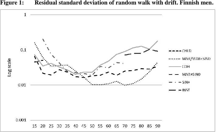
For each of the time series we also estimated a random walk with a drift model (RWD model), where is a deterministic drift and is an error term. In the cases where autocorrelation had been detected we compared the residual standard deviations estimated from the RWD model and the ARIMA model that gave the best fit. Although the RWD model did overestimate the residual standard deviation compared to the more refined model, the differences between the two were generally small. Striving for parsimony, we therefore decided to employ the RWD model throughout. This means that for a few household positions and age groups our prediction intervals for the household shares are wider than strictly necessary. In this sense our assessment of uncertainty is a bit conservative.
Figure 1: Residual standard deviation of random walk with drift. Finnish men.
Source: Own computations based on data supplied by Statistics Finland.
Note: The categories refer to the six fractions defined in Section 3.4.
We estimated the correlation between the sexes to be 0.46 for Denmark and 0.53 for Finland, assuming independence of age and household position. Based on the work on Norwegian data by Alho and Keilman (2010), we assumed an AR(1) model,
| | , for the correlation across age groups, assuming independence of sex and household position. Here refers to the errors from the random walk with drift models; = age, =sex, =time, whereas k=1, …, 6 refers to the six fractions defined above. The first-order autocorrelation was therefore estimated as the empirical correlation between residuals ̂ and
3.5 Simulation of household shares
We took 3000 draws, from a t-distribution.5 We assumed that the errors ̂ of RWD model for the fractions , k = 1,...6 have a normal distribution, with expected value zero, and standard deviation estimated from that model. The level prediction interval for is of the form
̂ ⁄ ̂ √
where is the number of observations in the RWD model, ̂ is the estimated drift, ⁄ is the ( ⁄ ) quantile of a t-distribution with degrees of freedom, and ̂ is the estimated residual standard deviation of the RWD model.
The terms and ⁄ under the square root account for innovation variance and for estimation error in the drift, respectively, while the t-distribution accounts for estimation error in the innovation variance.
Assuming standard deviation and correlation between the sexes and across age groups as estimated from the time series analysis, these are used to create correlated errors, for each sex and age group. These errors are then added to the point predictions from the deterministic household projection, which have been transformed into the same type of logit fractions as described in the previous section.
We then transformed the predicted shares in the logit scale back to shares in the original scale, for each time t and both sexes, according to:
⁄
⁄
5 The number 3000 for our household simulations was chosen for practical reasons only: the probabilistic
⁄
⁄
⁄
This way we obtained 3000 sample paths for each of these shares, specific for age and sex. Finally, we multiplied each of these sample paths for the household shares with one of the simulations from the stochastic population forecast. This then results in 3000 sample paths for the number of people in each household position.
Implicit in this multiplication is the assumption that the household shares and the population numbers are independent random variables. This assumption is difficult to check empirically, but we have reasons to believe that it is a reasonable one. A possible dependence is that between the number of elderly persons (which is determined by mortality) and the share of one-person households in that age bracket. Often, when one of two partners in an elderly couple dies, the surviving partner becomes a one-person household. The implied correlation is likely small, because it refers to a second-order effect, namely the difference between mortality of men and women who live in a couple.
4. Data and assumptions
As mentioned above, we have used data on the population broken down by five-year age group, sex, and household position from population registers compiled by Statistics Denmark and Statistics Finland for January 1st of the years 1987–2008 and 1982–2007, respectively6.
We have also used data on transitions between household positions, broken down by sex and five-year age groups. These data show the number of persons who were in household position k (k=1,…,7) on 1 January of a certain year and in household position j (j=1,…7) on 1 January of the previous year. In this case we had Finnish data for the period 2004–2008 and Danish data for the period 2002–2006. The household transition data were used to compute one-year transition probabilities. We decided to use averages over the period 2004–2008 for Finland and 2002–2006 for Denmark so as to avoid erratic patterns for infrequent transitions. The probabilities of entry into single fatherhood in Finland seemed too high, and were therefore set to 20% of the corresponding numbers for women (but this probability was set to zero for men aged 10–14). The Finnish birth rate for single mothers in the age group 15–19 also seemed unrealistically high and was adjusted downwards to the Danish rate. In addition, for both countries the probabilities for entry to single parenthood after age 70 were set to zero, and those for going from single parent to other private households were set to 1. The same applies to dependent children after the age of 25.
Numbers of deaths, emigrants, and immigrants decomposed by age, sex, and household position, as well as births broken down by age and household position of the mother, were available for the same years as the rest of the transition data in the Danish case, whereas in the Finnish case they were only available for the year 2008. To avoid irregular patterns in Finnish age-specific death probabilities, the married, cohabiting, and single parents were combined into one group, and those living alone and those living in other positions in private households were gathered into another group. Similarly, the married, cohabiting, and single parents were grouped together when computing emigration probabilities.
Many of the age patterns for the transition probabilities are qualitatively the same for men and women and also between the two countries, although the magnitudes vary. As an example of the age patterns, Figures 2–5 show some of the one-year transition probabilities for Finnish women for the period 2004–20087.
Among the general features observed for both sexes and in both countries are:
6
For more information on the Danish data see www.dst.dk/declarations/761.
- young people who live on their own are likely to enter into cohabitation (Figure 2);
- those cohabiting in their 20s and 30s have high marriage probabilities (Figure 3);
- living with a spouse is a stable position except at the end of the life course when experiencing the death of the spouse or entry into an institution is common (Figure 4);
- for all age groups the cohabiting experience higher probabilities of switching to single household position than do those living with a spouse (Figures 3 and 4);
- young single parents often start a cohabiting relationship (Figure 5). When they are in their fifties they have an elevated chance of living alone because their (last) child leaves the household;
Figure 2: One-year transition probabilities. Women who live alone, 2004-2008, Finland
Source: Own computations based on data supplied by Statistics Finland.
As described above, what we have computed from the transition data are transition probabilities. What we need as input to our household projection model are, however, occurrence-exposure rates. Under a constant intensity assumption, the probability matrix is an exponential function of the rates matrix . Thus to find the occurrence-exposure rates in Mt we need to compute the logarithm of , defined as a power series.
The power series, however, does not always converge: see Van Imhoff and Keilman (1991: 77) for details. Hence we assume that the occurrence-exposure rate for a certain household event is equal to the one-year transition probability for the corresponding change in household position. This introduces a small error in the rates. Under the assumption used, a Taylor series expansion shows that the probability matrix and the rate matrix are related as ⁄ ⁄ , where is the identity matrix. Most rates are in the order of magnitude of a few per cent or less. Mortality at high ages is an exception, where rates up to 30% are found. Thus for mortality we computed rates from numbers of deaths and exposure times assuming that there are no disturbing events in the particular population group defined by age, sex, and household position.
0 0.05 0.1 0.15 0.2 0.25 0.3 0.35
10
-14
20
-24
30
-34
40
-44
50
-54
60
-64
70
-74
80
-84 90+
Pro
b
ab
ili
ty SIN0>COH
SIN0>MAR
SIN0>SIN+
SIN0>OTHR
Figure 3: One-year transition probabilities. Cohabiting women, 2004-2008, Finland
Source: Own computations based on data supplied by Statistics Finland.
Getting numbers for the institutional population in Denmark was difficult. A law was passed in 1987 which abolished the building of nursing homes from January 1st 1988. The existing nursing homes were to be phased out gradually. These were then to be replaced by nursing apartments which offer the same level of care, but where the residents all have their own apartment with bathroom and a small kitchen. The nursing apartments are not considered institutions in the legal sense. Although residents of these apartments are needs tested they are considered tenants, which involve a different set of rights and responsibilities compared to persons who live in an institution. As the nursing apartments are not considered institutions, those living there are not registered as living in an institution in the household register. The way the residents are registered can vary between municipalities.
0 0.05 0.1 0.15 0.2 0.25 0.3 0.35
10
-14
20
-24
30
-34
40
-44
50
-54
60
-64
70
-74
80
-84 90+
Pro
b
ab
ili
ty COH>SIN0
COH>MAR
COH>SIN+
COH>OTHR
Figure 4: One-year transition probabilities. Married women, 2004-2008, Finland
Source: Own computations based on data supplied by Statistics Finland.
For those living in nursing homes we have detailed information about numbers and transitions, broken down by age and sex. The data we have about the population living in nursing apartments are the numbers in the age groups 67–74, 75–79, 84–89, and 90+. We assume that the distribution across age and sex is the same in the nursing apartment population as in the nursing home population, which numbered about 10,000 and 30,000, respectively, in 2007. In order to get an estimate of the number of persons living in institutions in the jump-off population we therefore adjusted the distribution of residents in nursing apartments to fit into our age group classification and divided the residential population between the sexes using the age and sex distribution of the nursing home population in 2007. To accommodate the increase in the institutional population the numbers of elderly living alone were adjusted downwards. Although, as noted above, the registration of those living in nursing apartments varies between municipalities, we have reason to believe that the majority are registered as living alone. In the years when extra funding was given for the conversion and replacement of nursing homes we witness a steep decrease in the share living in nursing homes. This is mirrored by a sharp increase in the proportion living alone. The same is not the case for the share living with a partner.
0 0.05 0.1 0.15 0.2 0.25 0.3 0.35
10
-14
20
-24
30
-34
40
-44
50
-54
60
-64
70
-74
80
-84 90+
Pro
b
ab
ili
ty MAR>SIN0
MAR>COH
MAR>SIN+
MAR>OTHR
Figure 5: One-year transition probabilities. Lone mothers, 2004–2008, Finland
Source: Own computations based on data supplied by Statistics Finland.
As the Danish transition rates into institutions only reflected those moving to nursing homes, we decided to use the transition rates into institutions from the Finnish data in the Danish forecast.
0 0.05 0.1 0.15 0.2 0.25 0.3 0.35
10
-14
15
-19
20
-24
25
-29
30
-34
35
-39
40
-44
45
-49
50
-54
55
-59
60
-64
65
-69
70
-74
Pro
b
ab
ili
ty SIN+>SIN0
SIN+>COH
SIN+>MAR
Figure 6: One-year transition probabilities. People entering an institution, 2004–2008, Finland
Source: Own computations based on data supplied by Statistics Finland.
Figure 7: One-year transition probabilities. People leaving an institution, 2004–2008, Finland
Note: Different scale.
Source: Own computations based on data supplied by Statistics Finland.
0 0.05 0.1 0.15 0.2 0.25 0.3 0.35 70 -74 75 -79 80 -84 85
-89 90+
70 -74 75 -79 80 -84 85
-89 90+
Pro b ab ili ty SIN0>INST COH>INST MAR>INST OTHR>INST
Men
Women
0 0.005 0.01 0.015 0.02 70 -74 75 -79 80 -84 85
-89 90+
70 -74 75 -79 80 -84 85
-89 90+
Pro b ab ili ty INST>SIN0 INST>COH INST>MAR INST>OTHR
Multistate life tables based on the first projection interval, which is 2009–2013 and 2007–2011 for Finland and Denmark, respectively, give a summary view of the input rates for this period (Tables 1 and 2). Table 1 shows that the Fins spend a little more than a quarter of their lives living as a child, a third living with a spouse, 11% cohabiting, and around 20% living alone. The Danes spend a somewhat larger fraction of their lives living as a child and a little less living with a spouse (Table 2). Based on this life table the average Fin is more likely to be married than the average Dane; cf. below. In both countries the majority of children are born to mothers who live with a spouse, although the difference between births by married and cohabiting women is smaller in Denmark than in Finland.
Table 1: Percentage of lifetime spent in various household positions, and number of children by mother’s household position, Denmark 2007–2011
CHLD SIN0 COH MAR SIN+ OTHR INST All (=100%)
% years
Men 29 19 11 31 1 8 0.3 75.1
Women 26 21 11 30 5 6 0.7 79.9
children
0.02 0.08 0.70 0.83 0.08 0.16 0.00 1.88
The rates are held constant throughout the projection period, except for small changes due to consistency requirements; cf. Section 3.2. In Section 5.2 an alternative to holding the rates constant, based on trend extrapolation of the rates, will be discussed briefly.
Table 2: Percentage of lifetime spent in various household positions, and number of children by mother’s household position, Finland 2009–2013
CHLD SIN0 COH MAR SIN+ OTHR INST All (=100%)
% years
Men 26 20 11 35 1 6 1 74.8
Women 22 22 11 34 4 5 1 82.3
children
5. Results
5.1 Main outcomes8
The numbers of persons in each household position are obtained directly from multiplying the sample paths as described in Section 3.5. In addition we have computed sample paths for the number of private households of each type, as this is important for many planning purposes. The numbers of married and cohabiting households equal half the numbers of married and cohabiting persons. The number of other private households is estimated by dividing the population living in such households by 4.65, which was the mean size in Finland at the jump-off point. The same number was used for Denmark. Adding on the numbers of people living alone and single parents gives 3000 paths for the number of private households. Mean household size is then computed as the size of the population in private households divided by the number of private households.
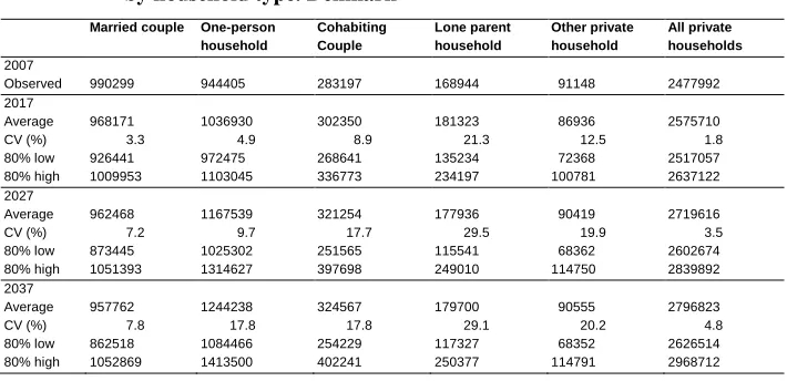
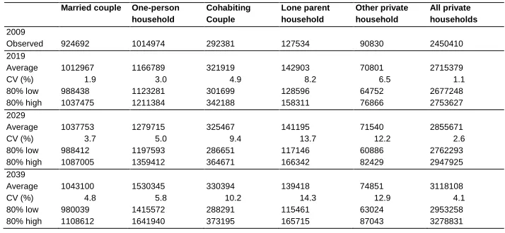
Tables 3 and 4 show the expected development in the number of private households of each type, the lower and upper bounds of the 80% prediction intervals, as well as the coefficients of variation (CV) for Denmark and Finland, respectively.
Table 3: Average value, coefficient of variation, and lower and upper bounds of 80% prediction intervals, for the number of private households, by household type. Denmark
Married couple One-person household
Cohabiting Couple
Lone parent household
Other private household
All private households
2007
Observed 990299 944405 283197 168944 91148 2477992
2017
Average 968171 1036930 302350 181323 86936 2575710
CV (%) 3.3 4.9 8.9 21.3 12.5 1.8
80% low 926441 972475 268641 135234 72368 2517057
80% high 1009953 1103045 336773 234197 100781 2637122
2027
Average 962468 1167539 321254 177936 90419 2719616
CV (%) 7.2 9.7 17.7 29.5 19.9 3.5
80% low 873445 1025302 251565 115541 68362 2602674
80% high 1051393 1314627 397698 249010 114750 2839892
2037
Average 957762 1244238 324567 179700 90555 2796823
CV (%) 7.8 17.8 17.8 29.1 20.2 4.8
80% low 862518 1084466 254229 117327 68352 2626514
80% high 1052869 1413500 402241 250377 114791 2968712
8
When we look at the growth in the numbers of private households of various types during the 30 year period, the strongest increase is expected in the number of one-person households: 31% and 50% in Denmark and Finland, respectively. We also notice quite a large increase in the number of households consisting of a cohabiting couple. On the other hand, the number of “Other private household” in both countries and the number of married couple households in Denmark will decrease slightly. Overall, we expect an increase in the number of Danish private households by 13%, from 2.5 to 2.8 million. For Finland we expect a growth of 27%, from 2.5 to 3.1 million. Married couple households become less important, numerically speaking, falling from 40% to 34% of all private households in Denmark and from 38% to 33% in Finland. The fraction of single person households, on the other hand, is expected to increase from 38% to 44% in Denmark and from 41% to 49% in Finland. It is virtually impossible that there will be fewer private households by 2037/2039: looking at the 3000 draws, only 1% of the Danish and none of the Finnish imply a smaller number of households in the final year than in the initial year. The corresponding number for married couple households is a staggering 67% for Denmark but only 0.7% for Finland. The probability of a decrease in single person households is 2% in Denmark, whereas in Finland none of the draws imply a reduction. All in all we expect a decrease in the average household size from 2.16 to 2.13 (80% prediction interval 2.01–2.28) in Denmark and from 2.14 to 1.89 (80% prediction interval 1.79–1.99) in Finland during the period.
Table 4: Average value, coefficient of variation and lower and upper bounds of 80% prediction intervals, for the number of private households, by household type. Finland
Married couple One-person household
Cohabiting Couple
Lone parent household
Other private household
All private households
2009
Observed 924692 1014974 292381 127534 90830 2450410
2019
Average 1012967 1166789 321919 142903 70801 2715379
CV (%) 1.9 3.0 4.9 8.2 6.5 1.1
80% low 988438 1123281 301699 128596 64752 2677248
80% high 1037475 1211384 342188 158311 76866 2753627
2029
Average 1037753 1279715 325467 141195 71540 2855671
CV (%) 3.7 5.0 9.4 13.7 12.2 2.6
80% low 988412 1197593 286651 117146 60886 2762293
80% high 1087005 1359412 364671 166342 82429 2947925
2039
Average 1043100 1530345 330394 139418 74851 3118108
CV (%) 4.8 5.8 10.2 14.3 12.9 4.1
80% low 980039 1415572 288291 115461 63024 2953258
We see that there is largest relative uncertainty, as reflected in the CVs, concerning the household types “Other private household” and “Lone parents”. The number of married couple households is easier to predict, as judged by the CV. The Danish predictions are more uncertain than the Finnish numbers. This is due to two reasons. 1. The Danish RWD models show somewhat larger residual standard deviations than the Finnish models. 2. Danish population numbers are somewhat more uncertain, especially among the elderly. For instance, 30 years ahead the CV for Danish men aged 95–99 is 0.83 compared to 0.62 for Finnish men. Likewise, for women the Danish CV is 0.61 and the Finnish 0.49. Note that forecasts for the total number of private households are more certain (CV-values after 30 years of 4.8% and 4.1% for Denmark and Finland, respectively) than forecasts for each of the specific household types (CV-values ranging from 4.8% to 29.1%). This is due to aggregation: some of the specific household types move in opposite directions. Hence their sum is easier to predict than the elements.
Note also that prediction uncertainty (still judged by the CV) increases more steeply during the first two decades than during the last decade of the forecast period. The reason that uncertainty stabilizes towards the end of the projection period is to be found in the transformation of the shares from the logit scale (with linearly increasing prediction intervals and unbounded predicted values) back to the original scale (with predicted values limited between zero and one).
With a few exceptions9, the coefficients of variation in Tables 3 and 4 are smaller than corresponding CVs for Norway in the article by Alho and Keilman (2010). Thanks to the high quality register data we were able to fit more realistic times series models (RWD) than Alho and Keilman: due to the paucity of their data they estimated very simple Random Walk models. If the real process is random walk with drift, a random walk model will result in too large estimates of the residual standard deviation.
While CVs reflect relative uncertainty, absolute uncertainty can be analysed by inspecting the width of the prediction intervals. The upper and lower bounds of the 80% prediction intervals in Tables 3 and 4 show that there is largest absolute uncertainty regarding the number of single person households in both Denmark and Finland. This reflects the fact that they are the most numerous household type. On the other hand, because of their small numbers, single parents have some of the smallest absolute uncertainties.
Figures 8 and 9 show that predicted household trends are in line with two broad developments that have gone on for a few decades: among all private households married couple households have lost their dominant position, while one-person households have become much more important, numerically speaking. This development, which also is to be found in many other Western countries (e.g.
9
Christiansen 2012), is caused by falling fertility and the increased popularity of consensual unions, combined with an increase in divorce. Since the late 1980s the shares of both cohabiting couple households and lone parent households have been remarkably stable.
Figure 8: One-person households, cohabiting and married couple households, and lone parent households, as a share of all private households. Observed (1987, 1997, 2007) and average projected values (2017, 2027, 2037), Denmark
Tables 5 and 6 contain the CVs for the number of people in different household positions for the age groups 20–24, 50–54, and 80–84, separately for each sex, for Denmark and Finland, respectively. The relative uncertainty is generally largest for the youngest age group. A notable exception is the group of young adults who live in consensual union, those in Denmark in particular. Although residual standard deviations for young adults are higher than those for middle-aged adults (cf. Figure 1 for the example of Finnish men), the large numbers of cohabiting young adults reduce their relative uncertainty. For the youngest two age groups (20–24 and 50–54) the greatest relative uncertainty concerns single parents. For the oldest age group there is a large amount of uncertainty concerning the cohabiting, the number living in nursing homes, and the number living in other private households. For the youngest age group
0 0.1 0.2 0.3 0.4 0.5
One person households
Cohabiting couple households
Married couple households
Lone parent households
1987
1997
2007
2017
2027
there is generally least uncertainty regarding the number of cohabiting and those living alone, whereas for the middle aged and elderly the most certain are the married and those living alone. In general, when there are many persons in a particular household position, this category is easier to predict than a less numerous one.
Figure 9: One-person households, cohabiting and married couple households, and lone parent households, as a share of all private households. Observed (1989, 1999, 2009) and average projected values (2019, 2029, 2039), Finland.
0 0.1 0.2 0.3 0.4 0.5
One person households
Cohabiting couple households
Married couple households
Lone parent households
1989
1999
2009
2019
2029
Table 5: Coefficient of variation for the number of people in different household positions for selected age groups, by sex. Denmark
20-24 years 50-54 years 80-84 years
Table 6: CVs for the number of people in different household positions for selected age groups, by sex. Finland
20-24 years 50-54 years 80-84 years
Men 2019 MAR SIN0 COH SIN+ OTHR INST 0.262 0.142 0.149 - 0.214 0.033 0.050 0.104 0.160 0.123 - 0.051 0.072 0.582 - 0.323 0.365 Men 2029 MAR SIN0 COH SIN+ OTHR INST 0.432 0.246 0.281 - 0.364 0.066 0.086 0.235 0.398 0.288 - 0.123 0.157 0.829 - 0.618 0.783 Men 2039 MAR SIN0 COH SIN+ OTHR INST 0.439 0.254 0.290 - 0.367 - 0.075 0.093 0.240 0.400 0.289 - 0.155 0.169 0.780 - 0.634 0.866 Women 2019 MAR SIN0 COH SIN+ OTHR INST 0.244 0.177 0.118 0.710 0.377 - 0.034 0.055 0.112 0.121 0.135 - 0.068 0.044 0.715 - 0.297 0.306 Women 2029 MAR SIN0 COH SIN+ OTHR INST 0.357 0.306 0.219 0.817 0.493 - 0.071 0.095 0.249 0.285 0.332 - 0.158 0.094 1.060 - 0.544 0.664 Women 2039 MAR SIN0 COH SIN+ OTHR INST 0.360 0.332 0.228 0.821 0.499 - 0.077 0.080 0.253 0.287 0.335 - 0.166 0.170 0.989 - 0.550 0.726
Figure 10: Box and whisker plots of the shares living in the household positions married, cohabiting, and living alone, men and women in selected age groups in 2037. Denmark
Married
Cohabiting
Figure 11: Box and whisker plots of the shares living in the household positions married, cohabiting, and living alone, men and women in selected age groups in 2039. Finland
Married
Cohabiting
5.2 Changing rates
As mentioned in Section 4, the input rates for the deterministic household forecast are held constant throughout the projection period, except for adjustments to satisfy internal and external consistency requirements. We tried to improve on this approach detecting a possible time trend in the rates. We assumed a linear trend in (the logit of) the rates and extrapolated these rates linearly. Thismeant that there were varying rates for each five-year period of the projection. Using these types of rates did, however, in some cases lead to implausible results. An example is the share of cohabiting among young (20–35) women in Denmark. Using varying rates led to a sharp increase in the share of these women from 2009 to 2019. The share then fell quite significantly from 2019 to 2029, and thereafter increased to about the same level as in 2019. In our opinion these results were implausible. For the majority of other household positions using varying rates did not have much effect on the results, and we therefore decided to stick to constant rates throughout the projection period. Loosely speaking, when rates are constant over time, this corresponds to shares that have constant (upward or downward) slopes.
5.3 RWD extrapolations
We also experimented with expected values for the shares computed from direct extrapolations of the random walk with drift models (transformed back from the logit scale to the original scale). This was done in order to directly take account of the trends in the shares. This approach did, however, in some cases lead to implausible results. For example, it gave results for Finland in 2037 where only around 60% in the age group 15–19 lived with their parents, and hardly any in the age group 20–24. In Denmark it all but extinguished the share of elderly living in other private households. Compared to the LIPRO findings, the results from this method suggest a much stronger substitution of marriage for cohabitation for the young and middle aged. An additional methodological drawback of this approach is that we cannot take advantage of the internal and external consistency requirements built into the LIPRO model.
6. Conclusion
horizon. Predictive distributions have been computed for households of several types and for persons in various household positions, including the institutionalized. We have used the random share approach developed by Alho and Keilman (2010), and tried to improve on their results by taking advantage of high quality data from Danish and Finnish population and housing registers. As was done in their article, we combined a probabilistic forecast for the share of people in each household position, broken down by age and sex, with simulations from a stochastic population forecast covering the same period. This then gives a probabilistic household forecast for the number of people in each household position.
Our results show an expected further increase in the number of private households, from 2.5 to 2.8 million (80% prediction interval 2.6–3.0 million) in Denmark and from 2.5 to 3.1 million (80% prediction interval 3.0–3.3 million) in Finland. Taken together with an increase in population size, this means a decrease in the mean household size from 2.16 to 2.13 persons per private household in Denmark and from 2.14 to 1.89 p/ph in Finland. We find a further reduction in the share of married couple households and a growing importance of one-person households. The largest coefficients of variation are for lone parent households and “other private household”, and smallest for married couple households. The single person household, on the other hand, displays the largest absolute uncertainty, reflecting the fact they are the most numerous household type.
How should users handle a specific forecast result in the form of a probability distribution, rather than one number? In the short term, up to five years, say, forecast uncertainty is not important. In the longer run, however, users should be aware of the costs attached to employing a forecast result that subsequently turns out to be too high or too low (“loss function”). Also, users should ask themselves whether an immediate decision based on the uncertain forecast is necessary, or whether they can wait for a while until a new forecast possibly shows less uncertainty. If an immediate decision is required they should try to determine the most essential features of the loss function, and base their decisions on that. For instance, will an overprediction imply the same loss as an underprediction of the same magnitude? If not, a number higher or lower than the median or the mean of the predictive distribution will be the optimal choice.
postponement of action. In other policy arenas greater uncertainty might indicate that the best polices would be those most easily changed as the future unfolds. For example, a planner of public care facilities facing uncertain projections of the number of elderly who need institutional care might decide to rent additional capacity rather than building or buying a new institution. Explicitly estimating the degree of uncertainty in demographic projections encourages consideration of alternative population futures and the full range of implications suggested by these alternatives (Lee and Tuljapurkar 2007).
The fact that we could use register data had several advantages, compared to the data of Alho and Keilman (2010). First, we could estimate all the transition probabilities without making approximations from data based on marital status and small sample surveys. Hence we obtained reliable rate estimates even for household events that occur quite seldom. Second, using register data implies that the same definitions (of households, families, etc.) have been used throughout. Third, the data, spanning more than 20 years in both countries, could be used to construct time series models of household shares. We could then analyse the empirical prediction errors in these time series models to derive estimates for the uncertainty in the predicted household shares. This is a clear improvement on the Alho and Keilman (2010) approach where the “uncertainty parameters were estimated from observed errors of an old household forecast against subsequent censuses”. The better data is reflected in the fact that, when it comes to household numbers, compared to the Norwegian results the vast majority of the coefficients of variation are smaller, given household position and number of years into the forecast.
Norway. But reliable estimates of such uncertainty measures require richer data than these authors disposed of.
Finally we want to stress a more general point. There are many reasons why administrative registers should get more emphasis in data collection for statistical purposes. An important one is that a traditional population census, based on questionnaires to be filled out by individuals, has become extremely costly to undertake. As an alternative many countries consider a change away from a traditional census to a register-based census. Countries such as Denmark, Finland, Norway, the Netherlands, and Sweden have shown how those registers can be used. The registers of Finland and the Netherlands have excellent household information, the quality of household data from Danish register is good (information on elderly institutions is not reliable), while Norwegian household data are problematic, due to problems in the dwelling register in that country. Statistical agencies should prioritize improving the quality of existing registers, and developing administrative registers in countries where they do not yet exist.
7. Acknowledgements
References
Alders, M. (1999). Stochastische huishoudensprognose 1998-2050 (Stochastic household forecast 1998-2050). Maandstatistiek van de Bevolking 11: 25–34. Alders, M. (2001). Huishoudensprognose 2000-2050: Veronderstellingen over
onzekerheidsmarges (Household forecast 2000-2050: assumptions on uncertainty intervals). Maandstatistiek van de Bevolking 8: 14–17.
Alders, M., Keilman, N., and Cruijsen, H. (2007). Assumptions for long-term stochastic population forecasts in 18 European countries. European Journal of Population 23(1): 33-69. doi:10.1007/s10680-006-9104-4.
Alho, J., Alders, M., Cruijsen, H., Keilman, N., Nikander T., and Quang Pham, D. (2006). New forecast: Population decline postponed in Europe. Statistical Journal of the United Nations ECE12(23): 1-10.
Alho, J., Cruijsen, H., and Keilman, N. (2008). Empirically based specification of forecast uncertainty. In: Alho, J., Hougaard Jensen,S., and Lassila, J. (eds.). Uncertain demographics and fiscal sustainability. Cambridge: Cambridge University Press: 34-54. doi:10.1017/CBO9780511493393.004.
Alho, J. and Keilman, N. (2010). On future household structure. Journal of the Royal Statistical Society: Series A 173(1): 117-143. doi:10.1111/j.1467-985X.2009. 00605.x.
Arminger, G. and Galler, H. (1991). Demografische relevante Modellrechnungen: Simulations- und Analyseverfahren auf der Basis empirischer Erhebungen. Materialien zur Bevölkerungswissenschaft Heft 72. Wiesbaden: Bundersinstitut für Bevölkerungsforschung.
Bell, M., Cooper, J., and Les, M. (1995). Household and family models: A review. Canberra: Commonwealth Department of Housing and Regional Development. Christiansen, S. (2012). Household and family development in the Nordic countries: An
overview. Paper presented at the International Seminar: Aging Households and the Nordic Welfare Model, Copenhagen, November 9-10 2012.
Fredriksen, D. (1998). Projections of population, education, labour supply and public pension benefits: Analyses with the dynamic microsimulation model MOSART. Oslo: Statistics Norway (Social and Economic Studies 101).
Galler, H. (1988). Microsimulation of household formation and dissolution. In: Keilman, N., Kuijsten, A., and Vossen, A. (eds.). Modelling household formation and dissolution. Oxford: Clarendon Press: 139–159.
Grundy, E., and Jital, M. (2007). Socio-demographic variations in moves to institutional care 1991–2001: A record linkage study from England and Wales. Age and Ageing 36(4): 424-430. doi:10.1093/ageing/afm067.
Højbjerg Jacobsen, R., Hougaard Jensen, S.E., and Rebbe, S.K. (2011). Husholdningsstrukturen i Danmark under forvandling: Betyder det noget for de offentlige udgifter? Nationaloekonomisk Tidsskrift 149(1-3): 109-125.
Jiang, L. and O’Neill, B. (2004). Toward a new model for probabilistic household forecasts. International StatisticalReview 72: 51–64.
Jiang, L. and O’Neill, B. (2006). Impacts of demographic events on US household change. Laxenburg: International Institute for Applied Systems Analysis. (Interim Report IR-06-030).
Jiang, L. and O'Neill, B.C. (2007). Impacts of demographic trends on US household size and structure. Population and Development Review 33(3): 567-591.
doi:10.1111/j.1728-4457.2007.00186.x.
Keilman, N., Kuijsten, A., and Vossen, A. (1988). Modelling household formation and dissolution. Oxford: Clarendon Press.
Keilman, N. and Brunborg, H. (1995). Household projections for Norway 1990-2020. Oslo: Statistics Norway. (Reports 95/21).
King, D. (1999). Official household projections in England: Methodology, usage and sensitivity tests. Geneva: Joint Economic Commission for Europe–EUROSTAT Work Session on Demographic Projections, Perugia, May 3rd–7th (Working paper 47).
King, M. (2004). What fates impose: Facing up to uncertainty, British Academy lecture.
http://www.britac.ac.uk/news/release.asp?NewsID=154.