Estimation of Static and Dynamic Demand Function of Household
Water in Qazvin Province and Review of the Rate of Change in
Consumer Behavior Over Time
S. Avazdahandeh1 S. Khalilian2
ARTICLE INFO Abstract:
Article history Received: 28/12/2018 Accepted: 07/07/2019
In this research, the demand function of drinkable water in Qazvin Province was estimated using dynamic and static methods. The required data were collected from the data of the provinces of Qazvin in the time period (1996-2016) and collected by referring to the statistical system of Statistics Center of Iran and the provincial planning and budget organization of Qazvin Province. The explanatory variables used in the model include household income, temperature (minimum and maximum), urban population, water price, rainfall, number of subscribers.
The method used to estimate the static model, generalized least squares, and in the dynamic model, is a two-step generalized moment method. The results showed that the water price coefficient in the static and dynamic model is -0.217 and -0.19, respectively, which is a negative sign of the correctness of the demand law and less than one indicative of the low elasticity of water. The variable coefficient of household income in the static and dynamic model was 0.2 and 0.15, respectively, which positive and less than one, respectively, indicating the normality and necessity of water in the drinkable sector. In relation to the price of other goods, the coefficient was estimated in both negative models were -0.72 and -0.9, respectively, which indicates that water is a complementary product. Finally, the value of the variable coefficient was 0.5, which indicates that the demand for water is 0.5 times the demand for water last year.
Keywords:
Dynamic Model, Static Model, Panel Data, Drinkable Water Demand Function.
1 Ph.D Student , Department of Agricultural Economics, Tarbiat Modares University.Corresponding author,
Email: [email protected].
2 Associate Professor, Department of Agricultural Economics, Faculty of Agriculture, Tarbiat Modares
Introduction
Over the past 100 years, cities have been receiving a large percentage of the world's population. According to United Nations forecasts, by the year 2030 more than 60% of the world's population will live in urban areas. Though cities occupy only about 2 percent of the Earth's surface, they hold more than half the world's population, rising at around 55 million tons a year. They consume three quarters of the world's resources and are the main producers of waste in the world (Egger, 2005). Urbanism can be defined as the expansion of a city, population growth, or the area of urban areas over time (Usha, 2002). Rapid urbanism threatens the sustainable life of the world with its negative effects on environmental parameters of water, air and soil (Todaro, 2006). On the other hand, with the expansion of cities, the need for water consumption will increase.
The problem is that Iran is in an arid and semi-arid region. The climate of Qazvin province is also semi-arid and the average annual precipitation is about 317 mm.
Table1. Statistical data of Qazvin province
Area (km) Population (people)
Distance from the center of the province (km) City Name 2031 63549 9.06 Abyek 0330 466643 56 Buin Zahra 330 666295 309 Alborz 9865 569646 -Qazvin 1906 426949 3303 Takestan 1852 34264 44603 Avaj
Source: Statistics Center of Iran
In the water year (2015-2016), the annual discharge from underground water sources is about 2010 million cubic meters, which has not changed compared to the water year in past but from the 408,000 items of water branch in the province, 290,000 items were associated with urban areas which has increased by 3.6% compared to last year (Qazvin province regional water company, 2016).
Table 2. Number of wells, discharge rate and household consumption in Qazvin province separated by city (Item-million cubic meters)
Number of wells (aqueduct) Discharge rate Household consumption City Name 669 ( 66 ) 646032 ( 6024 ) 404 Abyek 4646 ( 44 ) 296044 ( 64036 ) 405 Buin Zahra 3.4 ( 49 ) 426046 ( 4024 ) 4602 Alborz 6436 ( 4.4 ) 66606 ( 64042 ) 64064. Qazvin 45.4 ( 24 ) 344025 ( 9065 ) 904 Takestan ( 49 ) ( 6065 ) .095 Avaj
Source: Qazvin province regional water company
Table 3. Statistical mean of model variable separated by city
Abyek Buin Zahra Alborz Qazvin Takestan Avaj City Name/variable Name
0.1 404 206 62062 504 .035 Water consumption (million square meter)
103.8 64309 64309 64309 64309 64309
Water price index
52.6 6404 6404 6404 6404 6404 Household income (million rials) 162 694 4.. 665 644 455 Precipitation (Mm) 22.9 -4503 -4604 -4605 -4409 -4202 -Minimum temperature (Celsius) 33.5 3.04 3.05 3.05 3.06 4304 Maximumtemperature (Celsius) 22.9 4402 4606 44604 6402 604
Number of subscribers (1000 items) 93.1 3903 456 334 6504 606 Urban population (1000 people) 135.1 63606 63606 63606 63606 63606
The price index of other goods
Research Literature
In the context of estimating the demand function of water in the household sector, numerous studies have been carried out both inside and outside the country. Among them, we can mention the following:
Mohammadi and Akbari (2000) estimated the demand function of drinkable water in Kerman. They calculated the price elasticity of drinkable water demand between 0.17 and 0.36, indicating the low demand for drinkable water in relation to the price in this region, as well as the income elasticity was calculated between 0.01 and 0.12, indicating the indispensability of this good in the household basket. Pejouyan and Hosseini (2003) estimated the demand for water in the Tehran as demand price elasticity of 8% and 12%, and the demand income elasticity of 13% and 20% respectively, and in general, the low elasticity of household water demand in the Tehran city was confirmed. Sajjadifar and Kheyabani (2011) estimated the demand function of Arak household water. In general, the low elasticity of household water demand relative to income and price, as well as the completeness of water with other goods was confirmed.
Also, the results showed that the price elasticity and the income of the summer season (the successor to external costs) were almost twice the price elasticity and the income of the winter season (the successor to household consumption), and the long-term demand elasticity was calculated more short-term type. Adipour and Shirazshiani (2014) estimated the demand function of drinkable water in Golestan province. The results showed that the price elasticity of water demand is 0.26, income elasiticity is 0.95, and crossover price elasticity is 0.2, that is, water is a necessary and complementary good. The minimum water requirement for a Golestan subscriber was also achieved at a rate of 687 l/d.
Among foreign studies, the following cases can be mentioned: Hoglund (1999) in a study to estimate the household water demand function and to examine the effect of the potential tax on household water consumption in Sweden. The results showed that long-term price elasticity in the final price models was 0.1 and in the average price model of 0.2. The research findings indicated that the tax rate for one a currency (Kronor) for cubic meter of water consumption, which is roughly equivalent to a 5% increase in average water prices, would generate 600 million Kronor annual tax revenues, while water consumption decreases by 1%. Cader et al. (2004) conducted a research on the prediction of household water consumption under a blocked price structure in Kansas. In this study, they studied water consumption at macro level, while previous research was conducted at micro level. The results showed that water per capita consumption in eight areas is significantly different. The share of low consumption block is decreasing and high consumption block is increasing.
case of combined urban and household water demand, they are more elasticity to the price, but it is still no elasticity, that is to say, household water demand and urban water demand are successors together. The results also showed that household water consumption is influenced by factors such as the amount of the amount of water saved, supply infrastructure, income, and the social and economic characteristics of each community. Dharmaratna and Harris (2012) in a study to estimate the household water demand function in Sri Lanka. The results showed that the share of water consumption per month that did not show any sensitivity to price changes that was between 0.64 and 1.06. The results also indicated that reducing water use through the price tools in developed countries is more successful than developing countries. The price elasticity ranges from -0.11 to -0.14 and income elasticity ranges from 0.11 to 0.14. It is therefore concluded that policy makers in developing countries should not rely solely on price instruments to reduce water consumption. Andre and Carvalho (2014) conducted a study titled "Spatial Factors in Urban Water Demand in Fortaleza of Brazil".
They used three econometric models to achieve the research objectives. These models include Spatial Error Model (SEM), Spatial Autoregressive model (SAR) and Spatial Autoregressive Moving Average model (SARMA). The results indicate that the SARMA model is the best model in terms of time series tests.
The results obtained in this study are contradictory with previous studies, which means that among the other factors, these uncontrollable spatial factors are a key fault and ignoring the effects of almost all variables in the model.
Internal studies on the estimation of household water demand function
Estimation of demand for drinkable water in Kerman
Econometric method (The Stone–Geary utility function) Combined
data Mohammadi and
Akbari (2000)
Estimation of Household Water Demand Function (Case Study of Tehran) Econometric method
(The Stone–Geary utility function) Time
series data Pejouyan and
Hosseini (2003)
Estimation of Household Water Demand Function in Zahedan Econometric method
(The Stone–Geary utility function) Time
series data Khosh-Akhlagh
and Shahraki (2008)
Estimation of water demand function in Urmia
Econometric method (The Stone–Geary utility function) Time
series data Abdoli and Dizaji
(2009)
Modeling of Household Water Demand Using a Randomized Model Method, Case
Study: Arak Econometric method
(The Stone–Geary utility function) Combined
data Sajjadifar and
Kheyabani (2011)
Estimation of Golestan Water Demand Function
Econometric method (The Stone–Geary utility function) Time
series data Adippour and
Shirashiani (2014)
External studies on the estimation of household water demand function
Household demand for water in Sweden with implications of a potential tax on
water use Econometric
Combined data Hoglund (1999)
Estimating urban residential water demand determinants and forecasting water demand
for Athens metropolitan area Econometric method
(The Stone–Geary utility function) Time
series data Bithas and
Stoforos (2006)
Estimating household water demand using revealed and contingent behaviors:
Evidence from Vietnam Econometric
Combined data Cheesman et al
(2008)
Urban water demand for service and industrial use
Econometric Combined
data Arbués et al
(2010)
Estimating residential water demand using the stone geary functional form: the case of
Sri Lanka Econometric Time series data Dharmaratna and Harris (2012)
Spatial Determinants of Urban Residential Water Demand in Fortaleza Econometric Cross sectional data Andre and Carvalho (2014)
Analysing Household Water Demand in Urban Areas: Empirical Evidence from Faisalabad, the Industrial City of Pakistan Econometric
Cross sectional
data Ahmad et al
(2016)
By examining the these studies, it is clear that household water consumption is inversely related to the price and has a direct relationship with household income. The consumption with time-delay is also considered in this study using a dynamic model.
The theory of the function of household water demand The household water demand can be made in two ways:
1. Demand as input: Industrial and agricultural demand from water, as the optimal amount of it is derived from the condition of maximizing production relative to cost constraints.
(water as an essential goods and low elasticity). In order to extract the household water demand function, the principles of microeconomics and maximizing the utility of the consumer are used according to the budget. There are various utility functions in this direction, such as the Acanem, Klein-Rubin, and several other functions, such as the ideal AIDS function. The Acanem function is suitable for estimating non- essential demand function coefficients, although in some cases it is also used to estimate the demand for essential goods. Other functions are not suitable for estimating the water demand function. The proper function in these conditions is the Stone–Geary utility function. Stone- Geary uses the Klein-Rubin utility function as below (Hendeson and koa, 1980):
In the above equation is and and which is
the amount of consumption of goods i and Si are the minimum consumption of
goods I, and βi is the final share of goods i. Suppose there are two goods (i = 2):
water and other goods (w = water, g = goods) taken from the sides of the logarithm on the basis of the Neper number:
In order to achieve the household water demand function, the utility function of equation () is maximized to the budget limit as follows:
By forming a Lagrange function equal to zero, placing the first order derivatives, the function of household water demand is obtained
In equation (9), Qw is a water demand function that is a function of the water
price, the price of other goods, household income and other variables (xj),
from this equation, then the estimation of the model of the calculated coefficients will be the same elasticity.
Study area and required data
Required data including the spatial dimension of the cities of Qazvin province and the temporal dimension of annual data during the time interval (1996-2016) by referring to regional water, water and sewage companies, Qazvin Meteorological Organization and the Iranian Statistics Center has been collected.
The variables used to estimate the household water demand function include household income, urbanism, minimum and maximum temperature, precipitation, water consumption, number of subscribers and price index of water.
Analyze
Given that the data has a spatial and temporal dimension, a test must be made regarding the type of data to be panel or consolidation. According to table (1), the test probability value of F Limer is less than 5%, therefore the Null hypothesis based on the consolidation data is rejected.
Table 1. F Limer test
Test name Test probability value Results
F Limer test .0.. Panel data
In this study, two dynamic and static models were used to estimate the water demand function. After determining the type of data, the type of model should be investigated for both random effects and dynamic effects. In this regard, the Hausman test is used. As Table 2 shows, the test probability value in both static and dynamic models is less than 5%, so the Null hypothesis is rejected and the model has fixed effects.
Table 2. Hausman test
Test name Model Test probability value Results
Hausman Static .0.6 Fixed effect model
Hausman Dynamic .0.. Fixed effect model
Null hypothesis of this test is that the coextensive of variance in both static and dynamic models is more than 5%, so the Null hypothesis is accepted.
Table 3.Wald test
Test name Model Test probability value Results
Wald Static .096 Existence of variance coextensive
Wald Dynamic .054 Existence of variance coextensive
Of the other cases that violates the classical hypothesis, the self-correlation between distorted sentences are discussed in the static model using the Wooldridge test. The result of the test according to table (4) is that the it is rejected as Null hypothesis, since the test probability value is less than 5%, indicating that the distorted sentences are self-correlation
.
Table 4. Wooldridge test
Test name Model Test probability value Results
Wooldridge Static .0..6 Existence of correlation
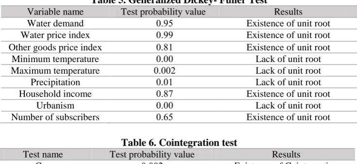
Table 5. Generalized Dickey- Fuller Test
Variable name Test probability value Results
Water demand .065 Existence of unit root
Water price index .066 Existence of unit root
Other goods price index .044 Existence of unit root
Minimum temperature .0.. Lack of unit root
Maximum temperature .0..6 Lack of unit root
Precipitation .0.4 Lack of unit root
Household income .042 Existence of unit root
Urbanism .0.. Lack of unit root
Number of subscribers .095 Existence of unit root
Table 6. Cointegration test
Test name Test probability value Results
Cao .0..6 Existence of Cointegration
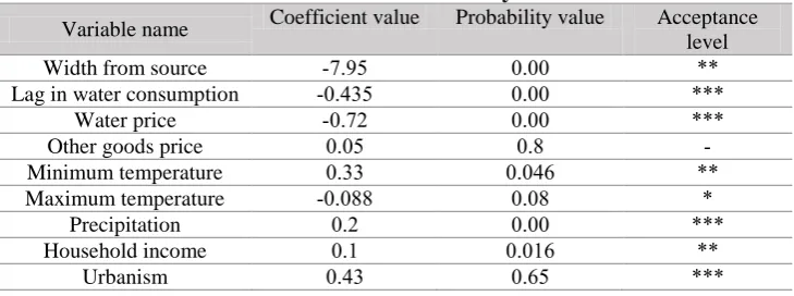
As stated in the previous sections, in this study the function of household water demand was estimated in both static and dynamic conditions. The superiority of the dynamic model to the static model is that the effect of the past behavior of the dependent variable is considered in the model, which is used in this study from a time lag. That is, the demand for water by citizens in this year depends on the size of the lag variable coefficient of demand for water in last year. The method used to estimate the static model is FGLS, since the Wooldridge test showed self-correlation in distorted sentences, which would no longer be required to resolve the distorted sentences. The results of Table 7 provide static estimation of the model. All coefficients in Table (7) represent elasticity marks, with the exception of the water price coefficient, which is twice the price elasticity of water. The price elasticity of water is estimated at 0.217, which is compatible with economic theories and previous studies. First of all, this elasticity is less than one, which implies the lack of water demand, and the negative is also the law of demand, meaning that by increasing the unit price of water, the demand will decrease by as much as 0.217. The price elasticity of other goods, which is considered as a goods and composite goods, has a value of 0.12, that is, firstly is negative, and secondly absolute value is less than one. The negative value indicates that the relationship between water and other goods is an complementary relationship, meaning that by increasing the unit price of other goods, the demand for water is reduced by as much as 0.12, while the decrease is lower than the price increase of other goods, and in fact it is a low elasticity product. The income elasticity of water demand was also calculated to be 0.2.
maximum temperature has a direct relation with water demand, so if it increases by one unit, water demand will increase by 0.33
Urbanism and the number of subscribers also have a direct impact on water demand, if any increases by one unit, water demand will increase by 0.1 and 0.43. The precipitation variable has an inverse relationship with water demand, so that if a unit increases, the water demand will decrease by 0.08.
Table 7. Estimation of static model by FGLS method
Variable name Coefficient value Probability value Acceptance level
Width from source -2065 .0.. **
Lag in water consumption -.0345 .0.. ***
Water price -.026 .0.. ***
Other goods price .0.5 .04
-Minimum temperature .044 .0.39 **
Maximum temperature -.0.44 .0.4 *
Precipitation .06 .0.. ***
Household income .04 .0.49 **
Urbanism .034 .095 ***
*show significantly at the level of 10%, ** show significantly at the level of 5%, *** show significantly at the level of 1%.
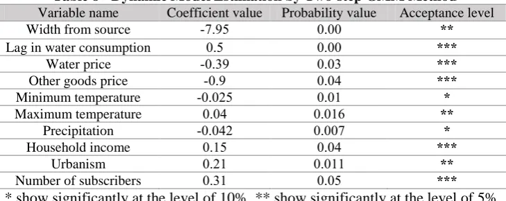
The results of the dynamic model are summarized in Table (8). The difference between this table and the table (7) is that the lag dependent variable is also included in the model and that the minimum temperature variable in this model is significant on the static model. The dynamic model is estimated using two-step GMM method. The advantage of this approach to the GMM method is to avoid the dependence between tool variables and distortion clauses. However, the Sargan test was used to test the existence of this correlation. As can be seen in Table (9), the probability of the Null hypothesis of this test is based on the lack of correlation of the tools with the remainder of more than 5%, so the Null hypothesis is accepted.
elasticity of water demand. On the other hand, the amount of water elasticity in the dynamic model is less than of the static model, which means that over time, the flexibility of water demand is lower than its price, and this decrease can be due to lack of suitable substitute for drinkable water and scarcity of this product over time. The price elasticity of other goods is 0.9, which like the static model is indicative of a complementary relationship between water and other goods. The amount of income elasticity of the demand for water is 0.15, which indicates the normal and essential water. Independent variables of maximum temperature, urbanism rate and number of subscribers had a direct effect on water demand, and the coefficients of each were estimated to be 0.04, 0.21 and 0.31, respectively. The other two independent variables, the minimum temperature and precipitation, also had a negative effect on water demand, so that by increasing each one unit, water consumption would decrease by 0.025 and 0.045.
Table 8 - Dynamic Model Estimation by Two-step GMM Method
Variable name Coefficient value Probability value Acceptance level
Width from source -2065 .0.. **
Lag in water consumption .05 .0.. ***
Water price -.046 .0.4 ***
Other goods price -.06 .0.3 ***
Minimum temperature -.0.65 .0.4 *
Maximum temperature .0.3 .0.49 **
Precipitation -.0.36 .0..2 *
Household income .045 .0.3 ***
Urbanism .064 .0.44 **
Number of subscribers .044 .0.5 ***
* show significantly at the level of 10%, ** show significantly at the level of 5%, *** show significantly at the level of 1%.
Table 9. Sargan test
Test name Test probability value Result
Sargan .064 Lack of correlation
Conclusions and Suggestions
than one and negative in both models, which indicates that the low elasticity of demand for water compared with the price of other goods, and the complementary relationship of water with other goods, meaning that water is no alternative good. Also, income elasticity in both the static and dynamic models had a value of less than one and a positive, indicating that the low elasticity of demand for water compared with the household income, and it is normal and necessary.
Finally, the coefficients in the dynamic model are less than the static state, and the its reason is the existence of a lag dependent variable that generates a portion of the variation of the independent variables to itself. The value of the coefficient of lag variation is a positive water demand, which states that water demand in t-1 period will have a direct and positive effect on water demand during t period.
Finally, by studying elasticity, we can propose methods for optimal water use in the household sector, which can be implemented by policy makers:
1. Price elasticity: the price elasticity of demand for water is less than one, that is, if the price increases, demand for it falls below the price. Therefore, price tools can be used to save on consumption.
2. Income elasticity: With this coefficient, subsidies paid to consumers can be tailored to the amount of optimal water demand. For example, if the government reduces its subsidy payments, household income will also decrease and demand for water will decrease.
3. Crossover price elasticity: The price of other goods can also be achieved with the goals of optimal water consumption. However, this is an approximate indicator because it is the product of combining hundreds of goods at different prices with a good and an approximate price.
4.Elasticity related to atmospheric factors: Considering the estimated coefficients, measures can be taken in relation to climate change. For example, when temperature rises, measures are to be taken to minimize the difference between the demand level of household customers and the amount of water resources.
5. Elasticity related to urbanism: By using a coefficient of urbanism, an interactive relationship between water consumption and population growth is obtained.
References
1- Adippour, M., and Shirashani, R., (2014). Estimation of Golestan Water Demand Function, Economic Modeling, 8 (26): 91-106.
2- Ashrafzadeh, S. H. R., and Mehregan, N., (2013), Econometric Panel Data, Cooperative Research Institute of Tehran University, Third Edition.
3- Ashrafzadeh, S. H. R., and Mehregan, N., (2014), Econometrics of the Advanced Data Panel, Nooreelm Publication, First Edition.
4- Pejouyan, J., and Hosseini, S., (2003). Estimation of Household Water Demand Function (Case Study of Tehran), Iranian Economic Research, 5 (16): 47-67.
5- Khosh-Akhlagh, R., and Shahraky, C., (2008). Estimation of Household Water Demand Function in Zahedan City, Economic Research, 8 (4): 129-145.
6- Qazvin Regional Water Organization. Office of Applied Research. Statistical Yearbooks (1996-2016).
7- Sajjadifar, S., Kheyabani, N., (2011). Modeling of Household Water Demand Using a Randomized Model Method, Case Study: Arak, Water and Wastewater, (3): 59-68.
8- Abdoli, Gh., and Faraji Dizaji, S., (2009). Estimation of water demand function in Urmia, Journal of Science and Development, 16 (28): 158-175. 9- Mohammadi, M., and Akbari, H., (2000). Estimation of demand for drinkable water in Kerman, Iranian economic research, 3 (7): 67-78.
10- Statistics Center of Iran, Statistical Yearbook of Qazvin Province, (1996-2006).
11- Ahmad SH et al .)1328( .Analysing Household Water Demand in Urban Areas: Empirical Evidence from Faisalabad, the Industrial City of Pakistan .
International Growth Center0
12- Andre D and Carvalho J 0)6.43( 0Spatial Determinants of Urban Residential Water Demand in Fortaleza, Brazil 0Water Resour Manage06343–63.4 ,64 ,
13- Arbués F, Ángeles M and Villanúa I (2010). Urban water demand for service and industrial use: The case of Zaragoza, Water resour manage, 24 (14):4033– 4048.
14- Bithas K and Stoforos CH (2006). Estimating urban residential water demand determinants and forecasting water demand for Athens metropolitan area,2000- 2010, South-Eastern Europe Journal of Economics, 1: 47-59.
15- Cader et al. (2004). Predicting household water consumption under a block price structure. Selected Paper prepared for presentation at the Western Agricultural Economics Association Annual Meeting, Honolulu, Hawaii, June 30-July 2, 2004.
17- Dharmaratna D, Harris E (2012) Estimating residential water demand using the stone-geary functional form: the case of Sri Lanka. Water Resour Manag 26(8):2283–2299.
18- Egger S. (2005). Determining a sustainable city model. Environmental Modelling & Software, 21, 1235-1246.
19- Greene, W. H. 2007. Econometric analysis. New york University. Sixth edition: 1-2.
20- Hendeson and koant (1980)
21- Hoglund L. (1999). Household demand for water in Sweden with implications of a potential tax on water use. Water Resources research, 35(12), 3853-3863.