Max Planck Institute for Demographic Research Konrad-Zuse Str. 1, D-18057 Rostock·GERMANY www.demographic-research.org
DEMOGRAPHIC RESEARCH
VOLUME 23, ARTICLE 9, PAGES 223-256
PUBLISHED 30 JULY 2010
http://www.demographic-research.org/Volumes/Vol23/9/ DOI: 10.4054/DemRes.2010.23.9
Research Article
Completing incomplete cohort fertility schedules
P.C. Roger Cheng
Eric S. Lin
c
°2010 P.C. Roger Cheng & Eric S. Lin.
2. Previous research 227
3. The U.S. fertility data 228
4. Specific estimation tactics 230
4.1 The APC framework 231
4.2 Out-of-sample period effects 232
4.3 Key to transforming a level into a schedule 233
4.4 A possible substitute for the actual CTFR 235
4.5 An illustrated example 239
4.6 Some remarks 241
5. Comparison among approaches 241
6. Summary and conclusions 249
7. Acknowledgements 250
Completing incomplete cohort fertility schedules
P.C. Roger Cheng1 Eric S. Lin2
Abstract
This paper develops a simple age-period-cohort framework in completing incomplete cohort fertility schedules, and makes full use of 1917–2005 U.S. data to obtain robust outcomes. Empirically, we indicate that the period effect is the key to transforming a fertility level into a fertility schedule. Accompanied by the smoothed version of tempo-variance-adjusted total fertility rates proposed in Kohler and Philipov (2001), we approximate the cohort fertility schedules fairly well and the estimates of all distributional parameters can be thereby obtained. Our approach is easy to implement and the data requirement is relatively light, indicating that the proposed method is readily applicable to countries whose data lengths are insufficiently long, and would be helpful for further empirical investigation of the relationship between cohort fertility behavior and other cohort-specific socioeconomic factors.
1Department of Economics, National Central University, Taiwan. No.300, Jhongda Rd., Jhongli City,
Taoyuan County 32001, Taiwan. Tel: 886-3-422-7151 ext. 66310; Fax: 886-3-422-2876. E-mail: [email protected].
1. Introduction
Childbearing decisions for a female to make include whether and when to have a child and how many children to have. From an aggregate perspective, the most comprehensive way to describe the fertility behavior of women in a birth cohort is to construct their complete fertility schedule, so that primary components of interest such as the level (quantum), the timing (tempo), and the variation (spread) can be directly derived. A cohort fertility schedule provides much useful and important information. The quantum of first births indicates the proportion of women who will have a child and that of all births tells us about how people reproduce themselves. In addition, the whole schedule reveals the distribution of the age gap between mothers and their children, which may influence the way they bring up the children and their ability in doing so, what kind of support parents can provide when their children are attending college, at what age parents will be when the children leave the nest, the financial aid that children can provide to support their parents when they are very old, and so forth. All these are interrelated with other life-cycle events including human capital investment, marriage formation and dissolution, labor force participation, and retirement. Moreover, a good understanding of fertility schedules also provides governments with a sound basis for population policies (e.g., pronatal interventions and tax reductions), social policies (e.g., family aid programs, pension benefits, and elder care programs), and health policies. If an increasing proportion of births are attributable to women of advanced maternal age (i.e., the fertility distribution becomes more skewed to the right), the government can therefore set up related policies for those women, because the changing pattern may have a significant public health impact due to the increased risks of stillbirth, preterm birth and cesarean delivery (see Joseph et al. 2005).
Measuring the actual childbearing behavior for cohorts, however, demands lengthy series of annual data. With a data set consisting of age-specific fertility rates (ASFRs) over a period of consecutive years (i.e., a Lexis rectangular surface of ASFRs), one can track cohorts diagonally over time and observe the changes in their fertility rates. If the series of annual data is lengthy enough, one will obtaincompletefertility schedules for several cohorts. Nevertheless, there are always a few cohorts whose fertility schedules
areincomplete, no matter how long the series is; data concerning their experiences while
younger or older are just not available.
that way be derived. For example, summing up all the observed and projected ASFRs of a particular cohort yields the estimated cohort total fertility rate (CTFR), and dividing these ASFRs by the estimated CTFR gives therelativeage distribution of fertility, from which one can compute the mean, the standard deviation, the coefficients of skewness and kurtosis, and so forth. For the use of some methods, data covering at least a few cohorts with a complete fertility schedule are required, and therefore such an approach may not be readily applied to countries whose data lengths are insufficiently long.
This paper develops a new approach to completing incomplete cohort fertility schedules, whose strategy is in essence different from that in previous research. Briefly, in previous studies the fertility level (i.e., the CTFR) was just one estimate among others generated from the projected ASFRs (i.e., the incomplete schedule), while we change the order of the estimation procedures, taking the fertility level as a crucial input for projecting the ASFRs. Our framework can operate well even when the data length is not too long, which broadens the range of its application. Furthermore, and most importantly, as will be shown in this paper, our approach outperforms previous methods in terms of forecasting incomplete cohort fertility.
Let us start with a broad description of the whole process, and then explain each elementary procedure in detail in subsequent sections.
The problem
• Suppose that an analyst has a set of 900 order-specific ASFRs for ages from 14 through 49 over a 25-year sample period ending in yearY (i.e., fromY−24through Y). This is an arbitrary set of times and ages, but it serves as a representative example of many real fertility data sets.
• The objective is to estimate the fertility schedule for the 60 birth cohorts (from Y −73throughY −14) bearing children during the sample period.
• The available data set spans the years{Y−24, . . . , Y}, while the observed cohorts bear children over the years{Y −59, . . . , Y + 35}. Therefore, the analyst needs some method to extrapolate ASFRs 35 years beyond the data set, both backward and forward in time.
The proposed estimation procedure to complete the incomplete cohort fertility schedule can be summarized in four steps as shown below and will be explained in more detail in Section 4:
General estimation strategy
1) Apply a simple age-period-cohort (APC) model to estimate age-, cohort-, and period-specific effects from the 25 years of sample data.
3) Fit out-of-sample period effects in a model that uses estimated CTFRs as control totals.
4) Fill in missing data by adding the in-sample age and cohort effects to the out-of-sample period effects.
Empirically, we indicate that the model for out-of-sample period effects in step 3 is the key to transforming a fertility level into a fertility schedule. With such a model, once
theactualfertility levels of cohorts who have not finished childbearing are known, their
incomplete fertility schedules can be estimated extremely well. Although the actual value of the CTFR is, in reality, not available, our research provides a possible substitute for it; smoothing the values of adjusted period fertility indicators can remove fluctuations in them and then summarize the trend, which becomes a good approximation to the CTFR.
Regardless of the forecasting approach adopted, accuracy should be a major criterion for any forecast worthy of the name. To test the predictive power of a model, we calculate
ex anteprojections based on a proportion of the whole data set we have and then compare
them with actual data. Moreover, since the results of testing the predictive power of a model may depend on the choice of prediction period, it is suggested that ex ante projections should be evaluated in a few periods rather than in just one particular period (see De Beer 1985:529). This paper makes as full use as possible of the long span in the U.S. data: we set a fixed subperiod length, move the starting point of the subperiod along calendar years, compute forecasts of competing approaches in each subperiod, and then assess their performances in all subperiods. In fact, the 1917–2005 U.S. data set is a good test for our method, because it includes not only 1) cohorts who experienced the postponement of childbearing, but also 2) cohorts who experienced the advancement of childbearing, and 3) cohorts who experienced the transition from the advancement to the postponement of childbearing.
2. Previous research
Given a data set consisting of ASFRs over a period of consecutive years, how can we complete the incomplete fertility schedule for women of a particular birth cohort whose childbearing information is censored at a young age, say 24? In this section we will review several (but not all) representative approaches to forecasting incomplete fertility, and their performances will be evaluated in Section 5.
The first and most simplified method assumes that the ASFRs at ages 25-49 from the last years in the data range will hold in the future. However, there is no guarantee that the cohort will necessarily follow this particular pattern. We refer to this method as the Naive approach hereafter.
The second approach fits a parametric curve (a function of age) to approximate the cohort’s ASFRs at younger ages (such as 14-24) in terms of some parameters, and then uses the estimated parameters to extrapolate the ASFRs at older ages (such as 25-49). Several curve fitting models have been proposed and utilized in forecasting incomplete fertility. For example, Bloom (1982) and Chen and Morgan (1991) used a modified version of the Coale and McNeil (1972) double exponential model
f(a) = .1946Θ
µ exp
½ −.1740
µ (a−a0−6.06µ)−exp
· −.2881
µ (a−a0−6.06µ)
¸¾
(where f(a) denotes the ASFR at age a, and Θ, µ, and a0 are parameters to
be estimated) to forecast the U.S. first births for incomplete cohorts. By contrast, Chandola, Coleman, and Hiorns (1999) adopted the Hadwiger function
f(a) = ρσ
τ
³τ
a
´3/2 exp
n −σ2³τ
a+
a τ −2
´o
(wheref(a)denotes the ASFR at agea, andρ,σ, andτare parameters to be estimated) to fit period (rather than cohort) fertility curves for a number of European countries. Yet the Hadwiger function is readily applied to forecasting cohort fertility.
Principal component models with time series extrapolation are considered in this paper as the third approach in forecasting fertility. The most prominent example is the Lee-Carter model (Lee and Carter 1992)
lnf(a, p) =δa+ηaκp+εa,p,
extrapolatedκp, one can thereby forecast the incompleted ASFRs for young cohorts.3 Note that the Lee-Carter method uses only the first component, while one can use several components to allow for greater flexibility in forecasting change, a strategy adopted in many studies (e.g. Booth, Maindonald, and Smith 2002; Renshaw and Haberman 2003).
We consider the methods proposed in Willekens and Baydar (1984) and Evans (1986) as the fourth and fifth approaches. The former decomposes ASFRs into age, period, and cohort effects, and utilizes time series methods to extrapolate period and cohort effects outside the data range, thereby forecasting incompleted ASFRs for young cohorts. The latter uses a linear regression model to predict the ASFRs after age 25. For each age between 25 and 39, the Evans method uses completed fertility data from earlier cohorts to estimate the coefficients of two predictors: 1) the cumulated cohort fertility through age 24 (quantum), and 2) the ratio of fertility at ages 15–19 to that at ages 20–24 (tempo), and then predicts corresponding ASFRs for young cohorts. As for ages 40-49, Evans “freezes” the ASFRs as they are in the last year of the data range.
To save space, we do not proceed to review other approaches. Although there are still several methods not mentioned in this section, the ones reviewed here can be considered to be important paradigms. For a comprehensive review of approaches and developments in demographic forecasting from 1980 to 2005, the reader can refer to Booth (2006).
3. The U.S. fertility data
The 1917–1980 U.S. age- and order-specific fertility rates are derived from Heuser (1976) and updated through 2005 from the Human Fertility Database.4 This data set provides
a time series of ASFRs for single years of age (from 14 to 49) according to birth orders (from 1 to 7 and 8+) covering most of the twentieth century. Also included are cumulative birth rates by cohort. From the whole data set, complete fertility schedules based on birth order can be constructed for cohorts 1903 (who were 14 in 1917) through 1956 (who were 49 in 2005), and corresponding distributional parameters such as percentiles or moments can thus be computed. The CTFRs are available even as far back as to cohort 1868 (who were 49 in 1917) since we also have cumulative birth rates.
3The framework developed in Li and Wu (2003) is a variant of the Lee-Carter method. They modeled fertility
for complete cohorts by age and cohort (rather than by age and period) and estimated the cohort-varying parameter using incomplete cohort observations (rather than applying time series methods).
4Human Fertility Database. Max Planck Institute for Demographic Research (Germany) and Vienna Institute
Figure 1: Cohort fertility quantum and tempo by birth order in the U.S. (a) (b) Birth Cohort C o h o rt T o ta l F e rt il it y R a te 0.0 0.5 1.0 1.5 2.0 1 8 6 8 1 8 7 8 1 8 8 8 1 8 9 8 1 9 0 8 1 9 1 8 1 9 2 8 1 9 3 8 1 9 4 8 CTFR1 CTFR2 CTFR3 CTFR4+ Birth Cohort M e a n A g e a t B ir th 20 24 28 32 36 1 8 6 8 1 8 7 8 1 8 8 8 1 8 9 8 1 9 0 8 1 9 1 8 1 9 2 8 1 9 3 8 1 9 4 8 MAB1 MAB2 MAB3 MAB4+
Note: The codesCTFRiandMABirefer to the cohort total fertility rate and the mean age at birth for birth
orderi∈ {1,2,3,4+}, respectively.
Figure 1 presents some order-specific fertility information in relation to cohorts as follows: 1) The CTFR decreased, then increased, and again decreased for cohorts 1868 through 1956 for all orders,5 as shown in panel (a). 2) The mean age at birth (MAB)
retreated, then advanced, and again retreated for cohorts 1903 through 1956 for all orders, as shown in panel (b). Trends in both panels look smooth.6
For illustration purposes, the following discussions will be restricted to the case of first births throughout this paper. Due to the fact that higher-order births (or other age-specific incidence rates such as first marriage) share the same data structure, our method can be directly applied to complete fertility schedules for higher-order births (or nuptiality schedules) without any difficulty.7 Instead of using all of the observations in 83 years
only once, our approach will be compared with others based on their performances in all subperiods of a chosen fixed length, thus making full use of the long span of the U.S.
5Due to the very small component of high birth orders in total fertility, data for birth order 4 and higher are
combined as order 4+.
6It should be noted that cohort indicators in this paper are computed with the use of period ASFRs rather than
cohort ASFRs. Although one may divide the period Lexis square into Lexis triangles under the assumption of a uniform distribution of childbearing within an age by period interval, as Willekens and Baydar (1984) did, the results obtained by these two methods are very close.
7An advantage of concentrating on first births is that our results can be readily compared with previous studies
data and yielding more robust results. Specifically, we mark any period of 25 consecutive years during 1917–2005 as a sample,8and there will thus be a total of 65 samples, from
the first one (1917–1941) to the last (1975–2005).
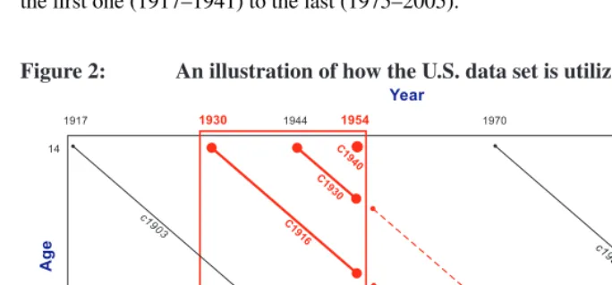
Figure 2: An illustration of how the U.S. data set is utilized
Figure2 illustrates the 1930-54 sample as an example, where ASFRs for 36 single years of age (from 14 through 49) covering 25 years (from 1930 through 1954) are available. Note that all fertility schedules for the 60 birth cohorts (from 1881 through 1940) covered in the 25-year data range are incomplete; data points are available only up to age 24 for cohort 1930. To derive complete fertility schedules for the 60 cohorts, the ASFRs at earlier ages for cohorts 1881–1915 and the ASFRs at older ages for cohorts 1906–1940 are required, which span the years 1895–1929 and the years 1955–1989.
4. Specific estimation tactics
In recalling that the general estimation strategy of our approach has been summarized into four steps in the Introduction, we now explain these steps in detail. In this section, we first exhibit the APC framework by which one can regress the ASFRs from the sample period on the age, period and cohort dummies, obtaining the corresponding within-sample estimates. We then show the reader how to use the CTFRs as an input in capturing the out-of-sample period effects, so as to estimate the ASFRs that fall out of the sample period. To put this procedure into practice, a smoothed Kohler-Philipov method is
8In this paper we choose 25 as the subperiod length because a 25-year ASFR data set can be obtained for many
proposed for obtaining estimates of the CTFRs. Furthermore, a concrete example is provided to illustrate our proposed estimation strategy.
4.1 The APC framework
Letf(a, p)represent the ASFR at agea∈ {14, . . . ,49}in periodp∈ {Y −24, . . . , Y}. One can establish an APC model and regress the 900 ASFRs within the sample period against 36 age dummies (A), 25 period dummies (P), and 60 cohort dummies (C) in a nonlinear least-squares way:9
f(a, p) = exp [ιβ+Aα+P ψ+Cγ] +νa,p, (1)
whereι is a vector of units, β denotes the intercept, and vectors α, ψ, and γ are the parameters of the age, period and cohort effects. The error term,νa,p, reflects age- and period-specific influences not captured by the model. To solve the identification problem arising from the linear dependence among the age, period, and cohort effects in Equation (1), we follow Deaton and Paxson (1994) by dropping one category from both setsAand C, respectively, and requiring that the coefficients of the period dummies sum to zero (Pψp= 0) and that they be orthogonal to a linear time-trend (
P
p ψp= 0).10
As is well known, there are numerous other identification strategies to choose from, such as equating the effect parameters of two cohorts (or two age categories), or applying the intrinsic estimator developed by Fu (2000) and further discussed by Yang, Fu, and Land (2004). Alternatively, one can follow Willekens and Baydar (1984) to quantify the effects of age, period and cohort with double classified data, so that the problem of identification will not arise. Different strategies will of course lead to different estimates of within-sample age, period and cohort effects.11 Nevertheless, in a way that
differs from most other studies applying APC models, this paper focuses on completing incomplete cohort fertility schedules rather than on identifying any individual effect of age, period or cohort. In Appendix 2, we provide a simple way to show mathematically that the identification strategy is irrelevant for the forecasting purpose. Furthermore, as we have investigated, estimates of the within-sample and the out-of-sample period effects by different strategies are almost identical after ridding them of a linear trend. As a
9For the derivation of the APC model, refer to Appendix 1.
10 The quality of fit of our APC model can be expressed by R2, which is defined as 1 −
SS(Residual)/SS(Total Corrected). Out of a total of 65 regression samples, 58 values ofR2are greater than
0.99 and the smallest of the other 7 values is 0.9886, showing that our model performs very well in explaining existing data in all samples.
11In the literature of demography, social science, and epidemiology, APC models have been widely used to
consequence, one may choose one’s favorite way to solve the problem without affecting the forecasting outcomes.
4.2 Out-of-sample period effects
Based on the APC model described in Equation (1), information regarding the out-of-sample period effects is necessary and crucial to extrapolate ASFRs beyond the sample range, so that the incomplete parts of fertility schedules can be constructed. An assumption concerning how period effects change outside the sample range is thus called for.
Given the 25 within-sample period estimates, an attractive option to think of is to utilize time series methods in extrapolating period effects outside the sample range, which is exactly the same idea that Willekens and Baydar (1984) adopted. However, how well does this approach work? Note that in more than half the samples, we do have actual ASFR data outside the sample range. Having obtained estimates of the intercept, the age and the cohort effects (i.e.,β,ˆ αˆandγ) in Equation (ˆ 1), out-of-sample period effects can be estimated using the following nonlinear least-squares regression:
f(a, p)/exp[ιβˆ+Aαˆ+Cγˆ] = exp[P ψ] +ua,p, (2)
wheref(a, p)is now the ASFR outside the data range,P denotes those out-of-sample period dummies, and the vector ψ captures the out-of-sample period effects.12 The
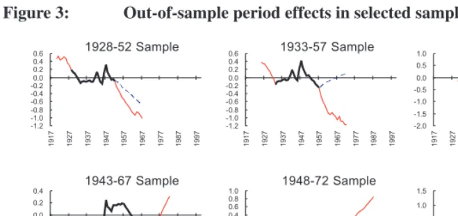
error term,ua,p, is added to capture particular influences besides the period effects. In other words, peeking at these outside data reveals theunknownperiod effects in selected samples, which are depicted in Figure3by thin lines extending from both ends of the
existingperiod effects (expressed by thick lines in the figure).
12In estimating the out-of-sample period effects, observations are discarded if the corresponding age is greater
Figure 3: Out-of-sample period effects in selected samples
Note: Thick lines denote the existing period effects within the datarange and thin lines extending from both ends represent the true but unknown out-of-sample period effects. Broken lines depict the estimated period effects using time series models.
Figure3also presents the time series projections by ARIMA models in broken lines for each selected sample, showing that the ambition of utilizing time series models might be frustrated owing to their salient deviations. As will be seen in Section 5., such deviations in out-of-sample period effects lead to poor performance in forecasting incomplete cohort fertility.
4.3 Key to transforming a level into a schedule
Since the ASFRs included within the data range are known and can be summed up for each cohort, the discrepancy in the sum from the CTFR represents the value to which the outside projected fertility rates should be summed up. Taking cohortc=Y −24whose childbearing information is available up to age 24 as an example,
CTFRY−24− 24 X
a=14
f(a, Y−24+a) = 49 X
a=25
f(a, Y−24+a). (3)
expressed as
f(a, Y −24 +a) = exp[ ˆβ+ ˆαa+ ˆγY−24+ψY+(a−24)], a= 25, . . . ,49, (4) where ψY+(a−24) denotes the out-of-sample period effect in period Y + (a− 24).
Rearranging Equation (3) as
49 X
a=25
exp£αˆa+ψY+(a−24) ¤
= CTFRY−24− P24
a=14f(a, Y−24+a) exp[ ˆβ+ ˆγY−24]
(5)
merely displays a loose relationship between the CTFR and the out-of-sample period effects, which is fruitless in completing the incomplete fertility schedule for cohortY−24
until a model characterizing the loci of out-of-sample period effects (denoted hereafter as
alocus function) is proposed.
In light of the “revealed” out-of-sample period effects shown in Figure3, one can first note that capturing how the out-of-sample period effects depart from the with-sample ones (backward and forward) is crucial. Next, we assume that the loci of out-of-sample period effects can be summarized as
ψY−24−x= Ψ( ˆψY−24, x;b0) or ψY+x= Ψ( ˆψY, x;b1), (6)
a function of 1) the estimated period effect at the nearest end of the existing data range
ˆ
ψY−24orψˆY, 2) the distance from that endx= 1, . . . ,35, and 3) adeparting direction parameterb0orb1, which can be precisely defined as
b0= ∂Ψ( ˆψY−24, x;b0)
∂x ¯ ¯ ¯ ¯ ¯ x=0
or b1= ∂Ψ( ˆψY, x;b1)
∂x ¯ ¯ ¯ ¯ ¯ x=0 .
Substituting Equation (6) into Equation (5) shows that once the value of CTFRY−24is
known, one can derive the departing direction estimateˆb1, compute the out-of-sample
period effects {ψˆY+1, . . . , ψˆY+35} by Equation (6), and obtain the projected ASFRs
outside the data range by Equation (4), thus completing the incomplete fertility schedule for cohortY −24.13
The locus functions mentioned in Equation (6) can be specified in infinitely many ways. Among others, the simplest can be a linear one:
ψY−24−x= ˆψY−24+b0x,
ψY+x= ˆψY +b1x.
13The same algorithm can be directly applied to cohorts {Y −38, . . . , Y −14}, whose fertility schedules are
However, a positive estimate ofbunder such a linear specification probably leads to some absurd situations in which the tail of a fertility schedule goes up rather than down. In order to prevent such cases, one may consider other specifications under which the locus becomes flatter as it moves farther from the end of the existing data range. For example, it can be a logarithmic one:
ψY−24−x= ˆψY−24+b0ln(x+ 1),
ψY+x= ˆψY +b1ln(x+ 1),
or a quadratic one:
ψY−24−x=
( ˆ
ψY−24+b0x ³
1− x
2ex
´
, if x= 1, . . . ,xe
ψY−24−x,e if x >x,e
ψY+x= (
ˆ
ψY +b1x ³
1− x
2ex
´
, if x= 1, . . . ,ex
ψY+ex, if x >x,e
where the locus is constrained to turn horizontally beyondexperiods.
In this paper, we adopt a quadratic specification withxe= 15as the locus function,14
and denote the estimated schedules so derived as APC-TRUE, for they are obtained from the collaboration of the APC framework with the true CTFR values.
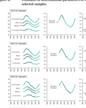
Figure 4 compares some estimates (including the mean, the median and the other two quartiles, the standard deviation, and the coefficients of skewness and kurtosis) of the APC-TRUE with the corresponding parameters in selected samples, demonstrating its excellent performance.15
4.4 A possible substitute for the actual CTFR
However excellent, the APC-TRUE is after all a hypotheticalmeasure since no actual CTFR for an incomplete cohort is available due to the data-range limitations. Can we then find a good substitute for the actual CTFR? This paper offers a possible one:
thesmoothed version of tempo-variance-adjusted period total fertility rates proposed in
Kohler and Philipov (KP; 2001).
14Since there can be infinitely many possible specifications, any particular one would be arbitrary andad hoc
in the absence of justification. Among the five specifications we have investigated (including the linear, the logarithmic, and the quadratic withex= 10,15,20), the projected fertility schedules derived from the quadratic (ex= 15) locus function with the actual CTFRs can best fit the true schedules on average.
15For reasons that will be explained in the next subsection, we focus on finishing an incomplete fertility schedule
Figure 4: Estimates in distributional parameters of the APC-TRUE in selected samples
Some methods are devised to correct the well-known distortions encountered by the period total fertility rate (PTFR; the sum of ASFRs during a particular year) as there exist changes in the age pattern of fertility. Bongaarts and Feeney (BF; 1998) proposed adjusting the PTFR by the change in the mean age at birth in adjacent years, based on the assumption that the shape of the order-specific age pattern of the ASFRs remains unvarying over time while the distribution may shift to higher or lower ages. Considering that constant shape assumption might be too strong, Kohler and Philipov extended the adjustment formula to include changes in the variance of the order-specific age pattern. Both methods work in terms of incidence rates which express births by order to women irrespective of their current parity, ignoring the fact that the tempo change not only affects the numerator but also the denominator of the ratio. Kohler and Ortega (KO; 2002), therefore, developed an approach which looks similar to the Kohler-Philipov method but works in terms of age- and parity-specific occurrence-exposure rates.
While quite a few researchers are skeptical about the usefulness of these adjusted period measures, due to their assumptions regarding the shape of the fertility schedules and/or due to their fluctuating and occasionally absurd values (e.g., Kim and Schoen 2000; Li and Wu 2003; Schoen 2004; Van Imhoff and Keilman 2000), some researchers have compared them with the CTFR (e.g., Kohler and Ortega 2002; Ryder 1990; Schoen 2004; Smallwood 2002; Sobotka 2003; Van Imhoff and Keilman 2000), explicitly or implicitly regarding these period indicators as forecasts of the completed fertility for cohorts who have not finished childbearing. In these studies, two popular ways of relating period and cohort fertility measures were adopted, namely, to compare the CTFR for cohortcwith the period estimate at time pat which the cohort reaches its mean age at birth (i.e.,c+MABc=p), or to compare the estimate at timepwith the CTFR for women who reach the mean age at birth in that year (i.e.,p−MABp =c). We follow the latter approach with a minor adjustment.
Given a 25-year sample period {Y −24, . . . , Y}, there will be only 23 KP figures obtained for years {Y −23, . . . , Y −1}; values for the first and the last years will not be available for reasons of calculation. The KP estimate in yearpis compared with the CTFR for cohortc=p−MABp. However, sinceMABpis in general not an integer, we interpolate the KP value for cohortc=p−MAB, whereMABis the average ofMABp over our entire data span from 1917 through 2005, rounded up or down to the nearest integer (for first birthMAB= 23).16
16This provides the reason, unexplained in the previous section, why we focus on filling out an incomplete
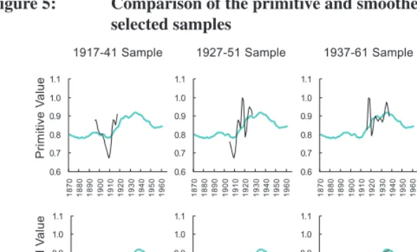
Figure 5: Comparison of the primitive and smoothed KP with the CTFR in selected samples
Note: The CTFR is depicted by a thick light line as a common background in all the panels, while the primitive and smoothed KP values are expressed by thin dark lines.
Panels in the first row of Figure 5 compare the (primitive) KP values with the corresponding CTFRs in selected samples. It is not unexpected that these values exhibit considerable fluctuations and some of them exceed the level of 1.0, just as discovered in previous studies.
What if we smooth the series of these fluctuating KP values? As is well known, smoothers are by definition devised to remove fluctuations and summarize the trends of data, and there have been a few studies (e.g., Currie, Durban, and Eilers 2004; Kohler and Philipov 2001; Silverman 1996) that smooth the original data before implementing their models. Since period fertility indicators often give rise to the problem of random fluctuations and the occurrence of impossible values while cohort-related parameters usually follow a smooth pattern, smoothing is then a reasonable choice. Panels in the second row of Figure5compare the smoothed KP values with the corresponding CTFRs in selected samples.17 Surprisingly, the approximation to the CTFR has been
consistently and significantly improved in all selected samples, and it can be convincing that the smoothed KP values indeed aid in forecasting the completed fertility for cohorts who have not finished childbearing.
4.5 An illustrated example
Having suggested the smoothed KP to serve as a possible substitute for the actual CTFR, we now take the 1930–1954 sample as an example to illustrate how our four-step estimation procedure works to complete the fertility schedule for cohort 1930 (who were 24 in 1954). As shown in Figure6:
Step 1. Use the APC model in Equation (1) to obtain the estimated within-sample
age, period and cohort effects.
Here we examine two strategies in solving the identification problem:
(ID-1) Set age 14 and cohort 1940 as reference groups, and require that the coefficients of period dummies be summed to zero and orthogonal to a linear trend
(ID-2) Set age 14 and period 1954 as reference groups, and require that the coefficients of cohort dummies be summed to zero and orthogonal to a linear trend
to show that 1) the within-sample and the out-of-sample period effects based on different strategies are almost identical after ridding them of a linear trend, and 2) the choice of identification strategy is irrelevant for forecasting purposes.
Step 2. Compute the smoothed KP values as an approximation to the CTFRs for
cohorts 1908–1930.18
Step 3. Produce estimates for out-of-sample period effects.
When identification strategy ID-1 is adopted, the departing direction estimates
ˆ
b0 = 0.0828andˆb1 =−0.1582, while if ID-2 is adopted, the departing direction
estimatesˆb0= 0.0769andˆb1=−0.1515.
Step 4. Combine the within-sample age and cohort effects in Step 1 with the
estimated out-of-sample period effects in Step 3 to derive ASFRs that fall out of the sample period and thus complete the cohort fertility schedule.
Note that the forecasted ASFRs are almost identical under identification strategies ID-1 and ID-2; we only depict the estimated schedule for the former and omit that for the latter.
The same procedure can be readily applied to other cohorts and other samples.
18 The S-PLUS program for calculating primitive KP values is available on Kohler’s website:
Figure 6: An illustrated example of how the estimation proceeds
Note: In Step 1, the?marks denote the reference group. In Step 3, points in the rectangular area (in broken
4.6 Some remarks
First, it is worthwhile emphasizing the structural differences between the forecasting strategies adopted in Willekens and Baydar (1984) and those in our new framework, although both methods are based on an APC model and stress the importance of forecasting the out-of-sample period effects. Willekens and Baydar forecast the period effects utilizing the existing period effects within the data range with a time series model, with the CTFR being merely an estimate among others generated from the projected ASFRs. Our method requires information on the CTFR from outside the APC model, which is then used as a crucial input for gauging in which direction the period effects will go and thereby projecting the ASFRs.
Second, it is necessary to be cautious that we do not attempt tomethodologicallyverify whether, from period fertility measures, we can infer cohort fertility. Instead, we share the view of Van Imhoff (2001:36) that “the justifiability of [period measures] can only be verified empirically”. The purpose of utilizing period measures in our context is simply to help estimate the out-of-sample period effects. We emphasize that there could be other possible substitutes for the actual CTFR. In fact, our APC framework is not limited to work with KP indicator but is ready to collaborate with any better method in forecasting the CTFR.
Furthermore, although the KO measure can be considered to be superior to the BF and the KP because it works in terms of occurrence-exposure rates rather than incidence rates, we focus our discussion on the KP approach in consideration of data availability, i.e., ASFR data are more available regardless of whether they are for developed or developing countries.
5. Comparison among approaches
To evaluate the performance of our APC framework accompanied by the smoothed KP, denoted as APC-KP hereafter, it is appropriate to find some rivals to compete with, according to the accuracy of projections in the incomplete age pattern of fertility rates. The approaches discussed in Section 2, including the Naive approach, the Coale-McNeil and the Hadwiger curve fitting models, the Lee-Carter method, the Willekens-Baydar method, and the Evans method, will be compared with the APC-KP.19 For reasons of
estimation, however, the 25-year data range is not long enough for the Lee-Carter method (some instability appears when the data length is less than 30 years) and the Evans method
19 The approach proposed by Li and Wu (2003) is excluded from the comparison because it requires data
to work. We thus grant the Lee-Carter method 5 additional years, and the Evans method 5 or 10 additional years (denoted as Evans-30 and Evans-35, respectively) in each sample as a premium. Again, in taking the 1930–1954 sample as an example, all approaches except for the Lee-Carter and the Evans methods make their projections based on ASFR data for the years 1930–1954, while the Lee-Carter and the Evans-30 methods are based on data for 1925–1954 and the Evans-35 method is based on data for 1920–1954. In addition, the APC-KP can estimate incomplete fertility schedules not only for young cohorts (whose future childbearing has not been realized yet) but also for old ones (whose early childbearing has been finished but is unavailable from the data), while some rival approaches are limited to forecasting incomplete parts for young cohorts only. The comparison is thus aimed at cohorts whose childbearing has not been realized, especially the cohort whose data points are available up to age 24 in the data range.
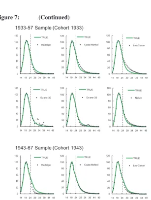
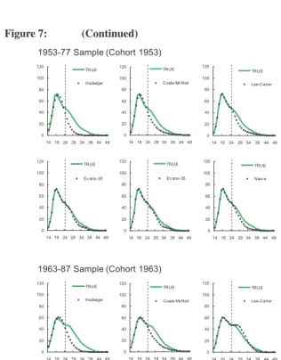
Figure 7 graphically illustrates the projections in incomplete fertility schedules by all approaches in selected samples, indicating that:
1. Although the rival approaches occasionally approximate the actual fertility schedules well (e.g., the Coale-McNeil, the Evans-30, and the Evans-35 in the 1943–1967 sample), they exhibit salient deviations in most cases.
2. The Coale-McNeil and the Hadwiger methods provide an unsatisfactory approximation of the empirical data, which is not unexpected for Henz and Huinink (1999) have demonstrated similar observations and attributed the outcomes to the censoring problem.
3. One may understand why the Lee-Carter and the Willekens-Baydar methods could produce large forecast errors, for their projections are based on time series models which might be unreliable because of a long forecast period or a structural change. 4. The Evans method displays a good approximation in the 1943–1967, the 1953–1977, and the 1963–1987 samples, but some absurd patterns and even negative projected values are found for the Evans-30 in the 1931–1955 and the 1933–57 samples.
5. Our APC-KP consistently performs well in all selected samples; its projections remain smooth and close to the actual fertility schedules.
24 in the yearY) in sample period {Y −24, . . . , Y}, the root mean square error (RMSE)
RMSE=
v u u t1
25 49 X
a=25 h
ˆ
f(a, Y−24+a)−f(a, Y−24+a) i2
(7)
is adopted as the criterion, where fˆandf denote projected and actual ASFRs (in live births per thousand women), respectively.
Figure8exhibits an overview of the performances in approximating the actual fertility schedule for three approaches (the APC-KP, the Evans-35, and the Naive) across 40 samples;20 the performances for other approaches are omitted for clarity because they
are even outperformed by the Naive. Based on the RMSE criterion, the figure shows that the APC-KP outperforms both the Evans-35 and the Naive with very few exceptions. It is worthwhile mentioning that the 1921–1945 sample is a special case in which the APC-KP performs badly (and so do other approaches), because there is an unexpectedly significant spike in the fertility rate at ages 25 and 26 for cohort 1921 (corresponding to the years 1946 and 1947) upon the return of the servicemen when the Second World War ended.
In addition to the RMSE criterion, one can also measure the proximity of an estimate (I) to the corresponding parameter (I) regarding a cohort fertility schedule with theˆ absolute percentage error (APE)
APE=|Iˆ−I|
I ×100% (8)
as the criterion, whereIcan be the CTFR, the mean, the median and the other quartiles, the standard deviation, the coefficients of skewness and kurtosis, and so forth. To evaluate the overall performances for all competing approaches, Table 1 presents the summary measures obtained from averaging the RMSEs and the APEs across 40 samples.21 Based
on the RMSE criterion in the ‘Schedule’ column, it is shown that the APC-KP method provides better projections of incomplete fertility schedules than all rivals. Moreover, the APC-KP estimates achieve the smallest deviation from most of the distributional parameters in terms of the APE criteria, except for the coefficients of skewness and kurtosis.22
20Note that it is not in every sample that the proximity of a schedule or its distribution-related parameters can
be evaluated, since the most recent complete fertility schedule that we have is for cohort 1956 (who were 49 in the year 2005). The last sample for which we can evaluate the performances of all competing approaches is the 1956–1980 sample.
21Measures of the hypothetical APC-TRUE are also included in the table as a benchmark.
22The Naive performs pretty well in projecting the coefficients of skewness and kurtosis, which is because its
Figure 7: Comparison of the estimated fertility schedules by previous approaches and the proposed APC-KP in selected samples
Figure 7: (Continued)
Figure 7: (Continued)
Figure 8: Performances of the APC-KP’s, the Evans-35’s, and the Naive’s schedule projections in 40 samples
6. Summary and conclusions
In this article, we develop a new framework in completing incomplete cohort fertility schedules, and the strategy adopted in the proposed method differs in essence from that in previous studies. In order to forecast incomplete fertility schedules, the traditional strategy is to utilize information contained in the existing ASFR data set to estimate the parameters of a particular underlying structure, and thereby to produce age-specific forecasts outside the data range. The cohort fertility level (i.e., the CTFR) is then simply a product generated from the projected schedule, as are estimates of other distributional parameters. On the contrary, we treat the CTFR as a crucial input for projecting the unknown ASFRs.
Specifically, we propose a simple age-period-cohort model to decompose age-specific fertility rates into age, period, and cohort effects. Empirically, our experiment indicates that the period effect is the key to transforming a fertility level into a fertility schedule; once the actual fertility levels of cohorts who have not finished childbearing are known, their incomplete fertility schedules can be estimated extremely well. In this paper we suggest that the smoothed version of tempo-variance-adjusted total fertility rates proposed in Kohler and Philipov (2001) can provide useful information on the fertility quantum, and the collaboration between our APC framework and the smoothed KP outperforms the rival methods, including the Naive approach, the Coale-McNeil and the Hadwiger curve fitting models, the Lee-Carter method, the Willekens-Baydar method, and the Evans methods, in approximating the incomplete cohort fertility schedules and other distributional parameters. All empirical results presented in this paper are fairly robust for we make efficient use of the 1917–2005 U.S. data. As an emphasis, our approach is easy to implement and the data requirement is relatively light, indicating that the proposed method is readily applicable to countries whose data lengths are not sufficiently long.
The success of our method in forecasting incomplete cohort fertility might lead us to make a bold suggestion that future research along these lines purely and simply focus on the projection of quantum. In this paper we exemplify the smoothed KP as a possible substitute for the CTFR. Readers are more than welcome to suggest other alternatives to collaborate with our APC framework. While the quadratic locus specification imposed to reveal the unknown period effects indeed works well in this article, we have noted that its specification is still somewhatad hoc. It would be interesting to see if we can find other possible specifications and obtain better results.
understanding of how the fertility behavior develops over the life course and what our future kinship patterns look like, thus providing governments with a sound basis for making policies from a cohort perspective. In addition, as Bongaarts and Feeney (2006) extended their previous method developed in 1998 to life-cycle events (first marriage and death) other than birth, our methodology possesses the same potential in extending the scope of application to all life-cycle events. For each event, one can apply the same framework, maybe with a few adjustments, to obtain cohort schedules and the corresponding estimates of distributional parameters. Furthermore, these cohort-specific estimates regarding various life-cycle events (such as human capital investments, labor force participation, marriage, fertility, divorce, retirement, and so forth) might be incorporated into empirical research on their causal relationship.
7. Acknowledgements
References
Bloom, D.E. (1982). What’s happening to the age at first birth in the United States? A study of recent cohorts. Demography19(3): 351–370. doi:10.2307/2060976.
Bongaarts, J. and Feeney, G. (1998). On the quantum and tempo of fertility. Population
and Development Review24(2): 271–291. doi:10.2307/2807974.
Bongaarts, J. and Feeney, G. (2006). The quantum and tempo of life-cycle
events. Vienna Yearbook of Population Research 2006: 115–151.
doi:10.1553/populationyearbook2006s115.
Booth, H. (2006). Demographic forecasting: 1980 to 2005 in review. International
Journal of Forecasting22(3): 547–581. doi:10.1016/j.ijforecast.2006.04.001.
Booth, H., Maindonald, J., and Smith, L. (2002). Applying Lee-Carter under conditions of variable mortality decline. Population Studies 56(3): 325–336. doi:10.1080/00324720215935.
Chandola, T., Coleman, D.A., and Hiorns, R.W. (1999). Recent European fertility patterns: Fitting curves to ‘distorted’ distributions.Population Studies53(3): 317–329. doi:10.1080/00324720308089.
Chen, R. and Morgan, S.P. (1991). Recent trends in the timing of first births in the United States. Demography28(4): 513–533. doi:10.2307/2061420.
Coale, A. and McNeil, D. (1972). The distribution by age at first marriage in a female cohort. Journal of the American Statistical Association 67(340): 743–749. doi:10.2307/2284631.
Currie, I.D., Durban, M., and Eilers, P.H.C. (2004). Smoothing and forecasting mortality rates.Statistical Modelling4(4): 279–298.doi:10.1191/1471082X04st080oa.
De Beer, J. (1985). A time series model for cohort data. Journal of the American
Statistical Association80(391): 525–530. doi:10.2307/2288465.
Deaton, A.S. and Paxson, C.H. (1994). Saving, growth, and aging in taiwan. In: Wise, D.A. (ed.)Studies in the Economics of Aging. Chicago: University of Chicago Press: 331–357.doi:10.3386/w4330.
Evans, M.D.R. (1986). American fertility patterns: A comparison of white and nonwhite cohorts born 1903–56.Population and Development Review12(2): 267–293. doi:10.2307/1973111.
263–278.doi:10.1080/03610920008832483.
Henz, U. and Huinink, J. (1999). Problems concerning the parametric analysis of the age at first birth. Mathematical Population Studies 7(2): 131–145.
doi:10.1080/08898489909525451.
Heuser, R.L. (1976).Fertility Tables for Birth Cohorts by Color: United States 1917–73. Rockville, MD: National Center for Health Statistics, dhew publication no. (hra) 76-1152 ed.
Joseph, K.S., Allen, A.C., Dodds, L., Turner, L.A., Scott, H., and Liston, R. (2005). The perinatal effects of delayed childbearing. Obstetrics and Gynecology 105(6): 1410–1418.doi:10.1097/01.AOG.0000163256.83313.36.
Kim, Y.J. and Schoen, R. (2000). On the quantum and tempo of fertility: Limits to the Bongaarts-Feeney adjustment. Population and Development Review26(3): 554–559.
doi:10.1111/j.1728-4457.2000.00554.x.
Kohler, H.-P. and Ortega, J.A. (2002). Tempo-adjusted period parity progression measures, fertility postponement and completed cohort fertility. Demographic Research6(6): 91–144. doi:10.4054/DemRes.2002.6.6.
Kohler, H.-P. and Philipov, D. (2001). Variance effects in the Bongaarts-Feeney formula.
Demography38(1): 1–16.doi:10.1353/dem.2001.0004.
Lee, R.D. and Carter, L.R. (1992). Modeling and forecasting U.S. mortality. Journal of the American Statistical Association87(419): 659–672. doi:10.2307/2290204. Li, N. and Wu, Z. (2003). Forecasting cohort incomplete fertility: A method and an
application.Population Studies57(3): 303–320. doi:10.1080/0032472032000137826. Martinelle, S. (1993). The timing of first birth: Analysis and prediction of Swedish first birth rates.European Journal of Population9(3): 265–286.doi:10.1007/BF01266020. Renshaw, A.E. and Haberman, S. (2003). Lee-Carter mortality forecasting with age-specific enhancement. Insurance: Mathematics and Economics33(2): 255–272.
doi:10.1016/S0167-6687(03)00138-0.
Ryder, N.B. (1990). What is going to happen to American fertility. Population and Development Review16(3): 433–454. doi:10.2307/1972831.
Schoen, R. (2004). Timing effects and the interpretation of period fertility.Demography
41(4): 801–819.doi:10.1353/dem.2004.0036.
Smallwood, S. (2002). The effect of changes in timing of childbearing on measuring fertility in England and Wales.Population Trends109: 36–45.
Sobotka, T. (2003). Tempo-quantum and period-cohort interplay in fertility changes in Europe: Evidence from the Czech Republic, Italy, the Netherlands and Sweden.
Demographic Research8(6): 151–214.doi:10.4054/DemRes.2003.8.6.
Trussell, J. and Bloom, D.E. (1983). Estimating the co-variates of age at marriage and first birth.Population Studies37(3): 403–416. doi:10.2307/2174506.
Van Imhoff, E. (2001). On the impossibility of inferring cohort fertility measures from period fertility measures. Demographic Research 5(2): 23–64.
doi:10.4054/DemRes.2001.5.2.
Van Imhoff, E. and Keilman, N. (2000). On the quantum and tempo of
fertility: Comment. Population and Development Review 26(3): 549–553.
doi:10.1111/j.1728-4457.2000.00549.x.
Willekens, F. and Baydar, N. (1984). Age-period-cohort models for forecasting fertility. The Hague: NIDI: 11–111. (Working Paper No. 45).
Yang, Y., Fu, W.J., and Land, K.C. (2004). A methodological comparison of age-period-cohort models: The intrinsic estimator and conventional
generalized linear models. Sociological Methodology 34(1): 75–110.
Appendix 1
Letg(a, c)represent the ASFR at ageafor women born in periodc. The life-cycle pattern in timing the arrival of their children can be viewed as a function of the average number of children born to them throughout their reproductive years. The CTFR for cohortcequals
CTFR(c) =
Z
g(a, c)da (9)
and the relative age distribution of fertility is denoted byg(a|c) = g(a, c)/CTFR(c)so thatRg(a|c)da= 1and
g(a, c) =g(a|c)CTFR(c). (10) Furthermore, we specifyg(a|c)as the product of two components:
g(a|c) =h1(a)h2(a, c), (11) whereh1 contains only the variablea, andh2 contains nothing else but all interaction terms betweenaandc.23 By substituting Equation (11) into Equation (10) and taking logs, we have
lng(a, c) = lnh1(a) + lnh2(a, c) + lnCTFR(c). (12) The problem that arises here is whether there is a simple and intuitive way to specify the interaction termlnh2. Sinceg(a, c) =f(a, p)also denotes the ASFR for women ageda in periodp=a+c, a function ofpcan in effect capture most interaction betweenaand
c, with a minor limitation that symmetric terms (such asa2candac2) share a common coefficient. Specifically, since any continuous function ofpcan be approximated by a polynomial using Taylor’s expansion, all expanded terms frompn= (a+c)n, except for
an andcn, are products ofaandcwith various power combinations. As a consequence,
the period term can be viewed as a structured (but incomplete) interaction between the age and the cohort terms. Unless the aforementioned limitation is severely violated,lng(a, c)
can be decomposed in another way:
lng(a, c) =H1(a) +H2(p) +H3(c)
or g(a, c) = exp [H1(a) +H2(p) +H3(c)] (13)
to replace that in Equation (12), whereH1,H2, andH3denote the age, period, and cohort effects, respectively. Note that there is no one-to-one correspondence for components in Equations (12) and (13).24
23It is of no use specifying another component containing only the variablecsinceRg(a|c)da= 1must hold
for allc.
24For example, ifH
2(p) =p3=a3+ 3a2c+ 3ac2+c3in Equation (13), then thea3term will be attributed
Appendix 2
To show that the choice of identification strategy is irrelevant to the forecasting purpose, consider two alternative data generating processes:
lnf(a, p) =H1(a) +H2(p) +H3(c) (model 1)
and
lnf(a, p) = [H1(a) +ka] + [H2(p)−kp] + [H3(c) +kc] (model 2) wherekis any real number. Sincep = a+c, there is no way to distinguish between model 1 and model 2 in the data, which is the standard APC identification problem.
Suppose that we know the value off(a, p)for cohortp−aat agea. Since one can always identifyH1,H2, andH3 up to the choice ofk, suppose that we also know the
functionsH1,H2, andH3, but that we do not knowk. The projected value of ASFR
f(a+t, p+t)fortperiods beyond the data range can thus be obtained according to model 2:
lnf(a+t, p+t) = [H1(a+t) +k(a+t)] + [H2(p+t)−k(p+t)] + [H3(c) +kc]
which is equivalent to that according to model 1:
lnf(a+t, p+t) =H1(a+t) +H2(p+t) +H3(c),