University of New Orleans University of New Orleans
ScholarWorks@UNO
ScholarWorks@UNO
University of New Orleans Theses and
Dissertations Dissertations and Theses
Summer 8-2-2012
Computational Scheme Guided Design of a Hybrid Mild Gasifier
Computational Scheme Guided Design of a Hybrid Mild Gasifier
You Lu
Follow this and additional works at: https://scholarworks.uno.edu/td
Part of the Heat Transfer, Combustion Commons
Recommended Citation Recommended Citation
Lu, You, "Computational Scheme Guided Design of a Hybrid Mild Gasifier" (2012). University of New Orleans Theses and Dissertations. 1526.
https://scholarworks.uno.edu/td/1526
This Thesis is protected by copyright and/or related rights. It has been brought to you by ScholarWorks@UNO with permission from the rights-holder(s). You are free to use this Thesis in any way that is permitted by the copyright and related rights legislation that applies to your use. For other uses you need to obtain permission from the rights-holder(s) directly, unless additional rights are indicated by a Creative Commons license in the record and/or on the work itself.
Computational Scheme Guided Design of a Hybrid Mild Gasifier
A Thesis
Submitted to the Graduate Faculty of the University of New Orleans in partial fulfillment of the requirements for the degree of
Master of Science in
Engineering Mechanical
By
You Lu
B.S. Central South University, 2009
August, 2012
ii
ACKNOWLEDGEMENT
It is my honor to take this opportunity to thank my advisor, Dr. Ting Wang, for his
guidance and support while I worked under him as a graduate student. None of this would be
made possible without Dr. Wang's hard work and dedication to his students and the University of
New Orleans. I would also like to thank Drs. Kazim M. Akyuzlu, Martin J. Guillot, and Carsie
A. Hall, III for being a part of my thesis committee.
I would also like to thank my fellow colleagues, students and researchers Monayem
Mazumder, Dr. Jobaidur Rahman Khan, Reda Ragab, Xijia Lu, Hank Long, III, Scott Richard,
and others from the Energy Conversion and Conservation Center (ECCC) for their help, support,
and valuable suggestions.
Again, I would like to thank my parents for their support during the years in which I was
pursuing my Master’s degree in Mechanical Engineering. In addition, I would like to thank my
older sister Xiuhong Bao. She has always been there for me during both good and bad times.
iii
TABLE OF CONTENTS
LIST OF FIGURES ... vi
LIST OF TABLES ... ix
NOMENCLATURE ...x
ABSTRACT ... xii
CHAPTER 1. INTRODUCTION ...1
1.1 Background ...1
1.1.1 Introduction of Coal ...1
1.1.2 Methods of Using Coal ...1
1.1.3 IGCC System Description...3
1.2 Literature Review...4
1.2.1 Clean Coal Technology ...4
1.2.2 Detailed Description of the Coal Gasification Process ...4
1.2.2.1 Pyrolysis ...5
1.2.2.2 Devolatilization ...6
1.2.2.3 Carbon Particle Combustion/Gasificatioin ...8
1.2.3 Particle Combustion Model ...9
1.2.4 Gasification Reactions Summary ...10
1.2.5 Introduction of Different Gasifier ...11
1.2.5.1 Fluidized Bed Gasifier (FBG) ...11
1.2.5.2 FBG Design Considerations ...15
1.2.5.3 Fluidization Velocity ...15
1.2.5.3.1 Minimum Fluidization Velocity of Packed Beds ………15
1.2.5.3.2 Minimum Fluidization Velocity of Fluidized Beds ………17
1.2.5.3.3 Calculation of Vmf ...20
1.2.5.3.4 Terminal Setting Velocity ...23
1.2.5.3.5 Calculation Results of Minimum Fluidization Velocity……… ...25
1.2.5.4 Review of FBG History ...27
1.2.5.5 Entrained Bed Gasifier (EBG) ...36
1.2.5.6 EBG Design Considerations ...42
1.2.6 Mild Gasification ...46
1.2.6.1 Wormser Mild Gasifier ...47
1.2.6.2 Introduction of IMGCC System...49
1.2.6.3 ECCC Mild Gasifier ...51
1.3 Motivation and Objectives ...53
2. CFD FORMULATION AND THEORY ...55
2.1Problem Statement ...55
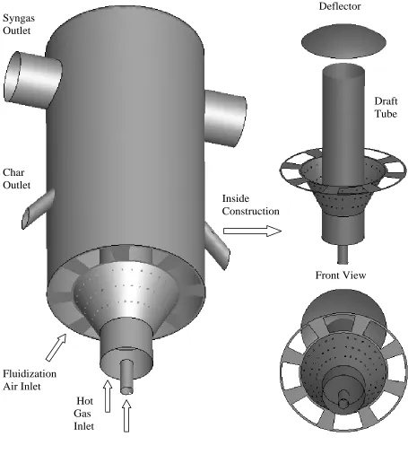
2.1.1 ECCC Mild Gasifier Design Consideration ...56
2.1.2 Description of Modified 2-D Gasifier Geometry ...58
iv
2.1.4 Description of Simulated 3-D Mild Gasifier Geometry ...61
2.2 Computational Model ...63
2.2.1 Physical Characteristics of the Problem ...63
2.2.2 General Governing Equations ...63
2.2.3 Turbulence Model ...65
2.2.3.1 Standard k-ε Model ...66
2.2.3.1.1 Standard Wall Function ...69
2.2.3.2.2 Enhanced Wall Function ...71
2.2.3.2 Other Models ...72
2.2.4 Radiation Models ...73
2.2.4.1 P-1 Radiation Model ...73
2.2.4.2 Advantages and Limitations of P-1 Radiation Model ...74
2.2.5 Chemical Reaction Model R ...75
2.2.5.1 Instantaneous Gasification Model ...75
2.2.5.2 Finite Rate Model ...79
2.2.5.3 Carbon Combustion Reaction Rates ...85
2.2.5.4 Coal Devolatilization Model ...88
2.2.5.4.1 Structural Models ...89
2.2.5.4.2 Empirical Models ...90
2.2.6 Boundary Conditions ...92
2.3 Computational Scheme ...97
2.3.1 Solution Methodology ...97
2.3.1.1 Preprocessing ...97
2.3.1.2 Processing ...97
2.3.1.3 Post-processing ...97
2.3.2 Computational Grid ...98
2.3.2.1 Grid Sensitivity Study for Case 3a ...103
2.3.3 Numerical Procedure ...103
2.3.4 Convergence Criterion ...109
2.3.5 Material Properties ...111
2.3.6 Patching Temperature ...111
2.3.7 Under-relaxation Factor ...112
3. MODELING MULTIPHASE FLOWS ...113
3.1 Introduction ...113
3.2 Multiphase Flow Regimes ...113
3.3 Approaches of Multiphase Modeling...115
3.3.1 Euler-Lagrange Approach ...116
3.3.2 Euler-Euler Approach ...116
3.3.2.1 The Volume of Fluid (VOF) Model ...116
3.3.2.2 The Mixture Model ...117
3.3.2.3 The Eulerian Model ...117
3.3.2.3.1 The Dense Discrete Phase Model ...118
3.3.2.3.2 The Wall Boiling Model ...118
3.3.2.3.3 The Multi-Fluid VOF Model ...119
v
3.4.1 Conservation Equations using Eulerian Multiphase Model ...120
3.4.2 Description of Momentum Equations ...122
3.4.2.1 Lift Forces ...122
3.4.2.2 Virtual Mass Force ...123
3.4.2.3 Inter-phase Momentum Exchange Coefficient ...124
3.4.2.3.1 Fluid-Fluid Momentum Equations ...124
3.4.2.3.2 Fluid-Solid Momentum Equations ...125
3.4.2.3.2.1 Solid Pressure...128
3.4.2.3.2.2 Radial Distribution Function...129
3.4.2.3.2.3 Solids Shear Stresses ...130
3.4.2.3.2.4 Granular Temperature ...132
3.4.3 Description of Energy Equations ...133
3.5 Multiphase Turbulence Models ...135
3.5.1 k-ε Mixture Turbulence Model ...136
3.6 Modeling Species Transport in Multiphase Flows ...137
4. RESULTS AND DISCUSSIONS ...142
4.1 Case 1 Fluidization Flow Behavior Study with Solid Particle ...143
4.1.1 Case 1a: Minimum Fluidization Velocity ...144
4.1.2 Case 1b: High Fluidization Velocity...146
4.1.3 Case 1c: A Moderated Fluidization Velocity ...147
4.2 Mild Gasification Simulation in ECCC Gasifier ...149
4.2.1 ECCC Mild Gasifier Design Considerations ...149
4.2.2 Case 2: Air-blown Mild Gasification (char chute exit pressure at 600 Pascal) ...150
4.2.3 Case 3a: Combusted Gas Blown at the Draft Tube and Syngas Blown at Fluidized bed ...159
4.2.4 Case 3b: Combusted Gas Blown at the Draft Tube and Volatiles Blown at Fluidized bed ...165
4.2.5 Case 4: 3-D Thermal-flow Behavior with Solids (no reaction) ...172
4.2.6 Case 5: 3-D Mild Gasification Simulation (Syngas blow at fluidized Bed)………..175
5. CONCLUSIONS...182
REFERENCES ...186
APPENDICES ...186
Appendix A Calculation of inlet gas mass fraction at the Draft tube Inlet ...193
Appendix B Calculation of molecular composition and enthalpy of formation of volatiles .. ...195
vi
LIST OF FIGURES
Figure 1.1 Schematic of Tampa Electri IGCC system (Source: DOE) ...3
Figure 1.2 Simplified global gasification processes of coal particles (sulfur and other minerals are not included in this figure). Heat can be provided externally or internally through combustion of char, volatiles, and CO ...5
Figure 1.3 Schematic drawing of Pyrolysis of Carbonaceous Fuels ...6
Figure 1.4 Schematic of fluidized bed gasifier (Source: Enggcyclopedia) ...12
Figure 1.5 Schematic of the High Temperature Wrinkler (HTW) Gasifier (Source: DOE) ...13
Figure 1.6 Schematic of a Kellogg-Rust-Westinghouse (KRW) gasifier. (Source: DOE) ...14
Figure 1.7 Schematic drawing of Minimum Fluidization Velocity ...19
Figure 1.8 Schematic of a downdraft an entrained bed gasifier (Source: Enggcyclopedia, http://www.enggcyclopedia.com/2011/12/gasification-processtypes/) ………...37
Figure 1.9 Schematic of the Shell gasifier ...38
Figure 1.10 Schematic of the General Electric gasifier ...39
Figure 1.11 Schematic of the Conoco-Phillips (E-Gas) gasifier (Source: DOE) ...40
Figure 1.12 (a) PRENFLO with Steam Generation (PSG) and (b) PRENFLO with Direct Quench (PDQ) ...41
Figure 1.13 Kellogg Brown & Root (KBR) transport gasifier ...43
Figure 1.14 Schematic of a counter-current moving-bed gasifier (Source: Enggcyclopedia, http://www.enggcyclopedia.com/2011/12/gasification-processtypes/) ...44
Figure 1.15 Schematic of the Lurgi pressure moving-bed gasifier (Source: DOE)………...45
Figure 1.16 Schematic diagram of a Mild Gasifier [Wormser (2008)] ...49
Figure 1.17 Schematic Diagram of an Integrated Mild Gasification Combine Cycle (IMGCC) System ...51
Figure 1.18 Schematic diagram of the cold-flow model of the ECCC Mild Gasifier ...52
Figure 2.1 Schematic of the 2-D Mild Gasifier ...60
Figure 2.2 Schematic of the 3-D simulated mild gasifier ...62
Figure 2.3a Boundary conditions for the 2-D Mild Gasifier ...93
Figure 2.3b Boundary conditions for the 3-D Mild Gasifier ...95
Figure 2.4a 2-D unstructured mesh (10,115 cells) of the 2-D mild gasifier ...99
Figure 2.4b 2-D unstructured mesh (21,582 cells) of the 2-D mild gasifier ...100
Figure 2.4c 2-D unstructured mesh (46,917 cells) of the 2-D mild gasifier ...101
Figure 2.5 3-D unstructured mesh (816,731 cells) of the 3-D mild gasifier ...102
Figure 2.6 Outline of the numerical procedures for the gaseous (primary) phase. The heterogeneous reaction (secondary) follows the similar process. Iterations proceed alternately between the primary and secondary phases...………...….108
Figure 2.7 Residuals for the transient ultimate case (Case 2: coal mild gasification (Note: Iterations before 830,500 steps are not shown for clarity.) ...110
Figure 4.1 Organization of simulated cases ...142
vii
Figure 4.3 Case 1b: 2-D transient distribution of volume fraction of carbon solid using 2.5 m/s fluidization air and 1 m/s in the draft tube inlet for time interval between 0.1 and 0.5 seconds. ...146
Figure 4.4 Case 1b: (a) velocity profile of air (b) velocity profile of carbon solid at 0.5 seconds ………147 Figure 4.5 Case 1c: Top row – 2-D transient distribution of volume fraction of carbon solid with 0.5 m/s fluidization velocity at horizontal inlet and 0.3 m/s velocity at the inclined surface inlet; Bottom row – (a) velocity profile of air (b) velocity profile of carbon solid at 0.5 seconds………...….……148 Figure 4.5 2-D transient distribution of (a) mass fraction of volatiles in gas phase and (b)
temperature of gas phase at t=2.0 seconds………..…….148 Figure 4.6 2-D transient distribution of (a) mass fraction of volatiles in gas phase and (b) temperature of gas phase at t = 2.0 seconds with 1 m/s coal feed speed…………..150 Figure 4.7a 2-D transient distribution of volume fraction of carbon solid with an emphasis within the draft tube for Case 2.. ...154 Figure 4.7b 2-D transient distribution of volume fraction of carbon solid with an emphasis on the fluidized bed for Case 2.. ...155 Figure 4.8 2-D transient distribution of mass fractions of various species at time t = 1.94 seconds for Case 2………..156 Figure 4.9 2-D transient distribution of mass fractions of volatiles (inside the coal) versus
volatiles (gas phase outside the coal) from 0.1 seconds to 1.94 seconds for Case 2 ………..157 Figure 4.10 2-D transient distribution of mass fractions of water vapor (inside coal) vs. water vapor (gas phase) from 0.1 seconds to 1.94 seconds for Case 2………...…….….158 Figure 4.11 Velocity vector plots for (a) particles and (b) air with corresponding particle and air temperature contours (K) at 0.58 seconds for Case 2. ...159 Figure 4.12 2-D transient distribution of mass fractions of various species at time t = 2 seconds for Case 3a ……….………162 Figure 4.13 2-D transient distributions of mass fractions of volatiles (in coal phase) vs. volatiles
(in gas phase) from 0.1 seconds to 2.0 seconds for Case 3a………...163 Figure 4.14 2-D transient distributions of mass fractions of water vapor (in coal phase) vs. water vapor (gas phase) from 0.1 seconds to 2.0 seconds (Case 3a)………164 Figure 4.15 2-D temperature distribution of (a) gas phase and (b) coal phase at t = 0.9 second. (Case 3a)………..….165 Figure 4.16 2-D transient distribution of mass fractions of various species at time t = 2 seconds for Case 3b………..167 Figure 4.17 2-D transient distributions of mass fractions of volatiles (coal phase) vs. volatiles
(gas phase) from 0.1 seconds to 2.0 seconds for Case 3b ...168 Figure 4.18 Transient distributions of mass fractions of volatiles (coal phase) vs. volatiles (gas
phase) from 0.1 seconds to 2.0 seconds (Case 3b) ...169 Figure 4.19 Distribution of mass fractions of volatiles (coal phase) vs. volatiles (gas phase) from
0.1 seconds to 2.0 seconds (Case 3b)………...170 Figure 4.20 Distribution of mass fractions of water vapor (coal phase) vs. water vapor (gas
viii
Figure 4.21 3-D transient distribution of the volume fraction of carbon solid from t = 0.2-2.0 seconds (Case 4) ...174 Figure 4.22 Transient distribution of the volume fraction of carbon solid at the mid-plane of the 3-D mild gasifier (Case 5)………177 Figure 4.23 A snapshot of the 3-D (a) velocity profile of the coal phase and (b) velocity profile of the gas phase at 0.3 seconds with the volume fraction of carbon solid being displaced in color (Case 5)……….….177 Figure 4.24 A snapshot of the transient distribution of the volume fraction of various gas species at the mid-plane of the 3-D mild gasifier at 0.9 seconds (Case 5)…………....…..178 Figure 4.25 Transient distribution of the mass fraction of volatiles within the gas phase in the mid-plane of the 3-D mild gasifier (Case 5)………...179 Figure 4.26 Transient distribution of the mass fraction of water vapor within the gas phase in the
ix
LIST OF TABLES
Table 1.1 Comparisons between combustion and gasification ...2
Table 1.2 Properties of the two phases ...26
Table 1.3 Summary of coal gasifier comparisons ...46
Table 2.1 Parameters, inlet and operating conditions for coal devolatilization reactions (Case 3 in Ch. 5)……….94
Table 2.2 Parameters, inlet and operating conditions for coal devolatilization reactions (Case 4 in Ch. 5)………...96
Table 2.3 Grid sensitivity study of Case 3a ...103
Table 4.1 Comparison of minimum fluidization velocity between those calculated from different correlations and that obtained from the CFD result for 0.25mm diameter and 0.6 volume fraction of carbon solid………...144
Table 4.2 Parameters, boundary and operating conditions for simulated Case 2 ...153
Table 4.3 Species composition at syngas exit at t = 1.94 seconds for Case 2 ...153
Table 4.4 Parameters, boundary and operating conditions for Case 3a………...161
Table 4.5 Species composition at syngas exit at t = 2.0 seconds for Case 3a...161
Table 4.6 Parameters, boundary and operating conditions for Case 3b ...166
Table 4.7 Species composition at syngas exit at t = 2.0 seconds for Case 3b ...166
Table 4.8 Parameters, boundary and operating conditions for Case 4 ...173
Table 4.9 Parameters, boundary and operating conditions for Case 5 ...176
x
NOMENCLATURE
a local speed of sound (m/s)
c concentration (mass/volume, moles/volume)
cp heat capacity at constant pressure (J/kg-K)
cv heat capacity at constant volume (J/kg-K)
D mass diffusion coefficient (m2/s)
DH hydraulic diameter (m)
Dij mass diffusion coefficient (m2/s)
Dt turbulent diffusivity (m2/s)
E total energy (J)
g gravitational acceleration (m/s2)
G linear-anisotropic phase function coefficient Gr Grashof number (L3ρ2gβ∆T/ µ2)
H total enthalpy (W/m2-K) h specific enthalpy (W/kg-m2-K) J mass flux; diffusion flux (kg/m2-s) k turbulence kinetic energy (m2/s2)
k thermal conductivity (W/m-K)
m mass (kg)
MW molecular weight (kg/kgmol)
M Mach number
p pressure (atm)
Pr Prandtl number (ν/α)
q heat flux
qr radiation heat flux
R universal gas constant (8314.34 J/Kmol-K)
S source term for mass, energy, species concentration
Sc Schmidt number (ν/D)
xi
t time (s)
T temperature (K)
U mean velocity (m/s)
X mole fraction (dimensionless)
Y mass fraction (dimensionless)
x, y, z coordinates
Greek letter
β coefficient of thermal expansion (K-1) ε turbulence dissipation (m2/s3)
εw wall emissivity
κ von Karman constant
µ dynamic viscosity (kg/m-s)
µk turbulent viscosity (kg/m-s)
v kinematic viscosity (m2/s)
v' stoichiometric coefficient of reactant v" stoichiometric coefficient of product ρ density (kg/m3)
ρw wall reflectivity
σ Stefan-Boltzmann constant
σs scattering coefficient
τ stress tensor (kg/m-s2)
Subscript
i reactant i
j product j
xii
ABSTRACT
A mild gasification method has been developed to provide an innovative clean coal
technology. The objectives of this study are to (a) incorporate a fixed rate devolatilization model
into the existing 2D multiphase reaction model, (b) expand the 2D model to 3D and (c) utilize
the improved model to investigate the mild-gasification process and guide modification of the
mild-gasifier design. The Eulerain-Eulerian method is employed to calculate both the primary
phase (air) and secondary phase (coal particles). The improved 3D simulation model,
incorporated with a devolatilization model, has been successfully developed and employed to
determine the appropriate draft tube dimensions, entrained flow residence time, The simulations
also help determine the appropriate operating fluidization velocity range to sustain the fluidized
bed depth without depleting the chars or blowing the char away. The results are informative, but
require future experimental data for verification.
Keywords: Clean coal technology, coal gasification, fluidized-bed, mild gasifier, CFD,
1
CHAPTER ONE
INTRODUCTION
1.1 Background
1.1.1 Introduction of Coal
China was the first country to utilize coal, alongside Greece and ancient Rome. The Greek scholar, Theophrastus, documented the nature of coal in the book "STONE" around 300 BC. The 12th century is when Native Americans started to use coal in their pottery industry.
Coal's formation is a continuous process. Coal is formed from the remains of vegetation that grew as many as 400 million years ago. It is often referred to as ''buried sunshine,'' since the plants which formed coal captured energy from the sun through photosynthesis to create the compounds that make up plant tissues and eventually become a part of the coal structure. The most important element in the plant material is carbon, which gives coal most of its energy. Most of the coal we are using right now was formed about 300 million years ago, when much of the earth was covered by steamy swamps. As plants and trees died, their remains sank to the bottom of the swampy areas, accumulating layer upon layer of biodegraded material and eventually forming a soggy, dense material called peat. Over long periods of time, the makeup of the earth’s surface changed, and seas and greater rivers caused deposits
of sand, clay, and other mineral matter to accumulate, burying the peat. Sandstone and other sedimentary rocks were formed, and the pressure caused by their weight squeezed water from the peat. Increasingly deeper burial and the heat associated with it gradually changed the material into coal.
1.1.2 Methods of Using Coal
2
liquefaction, coal is converted into liquid fuel. In gasification, coal is converted into synthetic gas (syngas).
Gasification is a process that converts any carbon-based materials, such as coal, pet-coke, biomass, or various wastes, into a synthetic gas (syngas) through an oxygen-limited environment. The clean syngas can be used as a fuel to produce electricity or valuable products such as chemicals, fertilizers, and transportation fuels. Compared to a combustion process that takes place in abundant oxidant conditions, a gasification process takes place under sub-stoichiometric conditions. Roughly, the amount of O2 used is only 35% or less of the amount required for complete combustion. The main
differences between combustion and gasification are listed in Table 1.1.
Table 1.1 Comparisons between combustion and gasification
Combustion Gasification
Occurs in excess-oxidant conditions Releases heat (exothermic)
Produces heat
Occurs in oxidant-lean conditions Less production of air pollutants gas Absorbs heat (endothermic)
Produces syngas
Gasification has a lower environmental impact compared to traditional combustion technologies because of the following reasons:
1. Gasification can recover the available energy from low energy density materials, such as municipal solid waste and pet-coke.
2. Syngas is cleaned before combustion, thus reducing air pollutants such as NOx and SOx.
3. By-products of gasification (sulfur and slag) are nonhazardous and marketable. 4. Higher efficiency.
5. Low CO2 production per kW of output due to higher efficiency.
6. Carbon dioxide (CO2) can be captured prior to syngas combustion. It gives the least costly and most
3
1.1.3 IGCC System Description
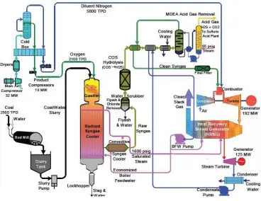
A very efficient way to use the syngas as fuel in electricity generation is by employing the Integrated Gasification Combined Cycle (IGCC). A schematic of a typical IGCC system is presented in Fig. 1.1. IGCC combines the gasification system with the gas clean-up system and the combined power system. The syngas produced by the gasifier is cleaned and used as a fuel for the gas turbines. The high-pressure and -temperature gases produced in the combustor then expand through the gas turbines to drive the air compressor and an electric generator. The hot exhaust gases from the gas turbines are sent to an HRSG (Heat Recovery Steam Generator), producing steam that expands through a steam turbine to drive another electric generator.
Integrated Gasification Combined Cycle (IGCC) also provides a more efficient method of capturing carbon dioxide (CO2) than in the conventional pulverized coal burning power plants. IGCC
demonstration plants have been operating since the early 1970’s and some of the plants constructed in the 1990’s are now entering successful commercial services.
4
1.2 Literature Review
1.2.1 Clean Coal Technology
Clean coal technology was dedicated to developing new and innovative technologies to reduce the negative impacts from utilizing coal for energy generation. If the coal is used as a fuel through combustion, SOx, NOx, CO2,and other trace elements (e.g., Hg and Ar), are generated by thermal
decomposition and released into air simultaneously. These emissions have been discovered to have a detrimental impact on the environment: e.g. acid rain and climate changes. Various clean coal technologies have been developed to reduce power plants’ emissions and increase their thermal efficiency. Among them, coal gasification technology possesses the greatest potential for achieving these goals. A detailed description of the coal gasification process and technology follows.
1.2.2 Detailed Description of the Coal Gasification Process
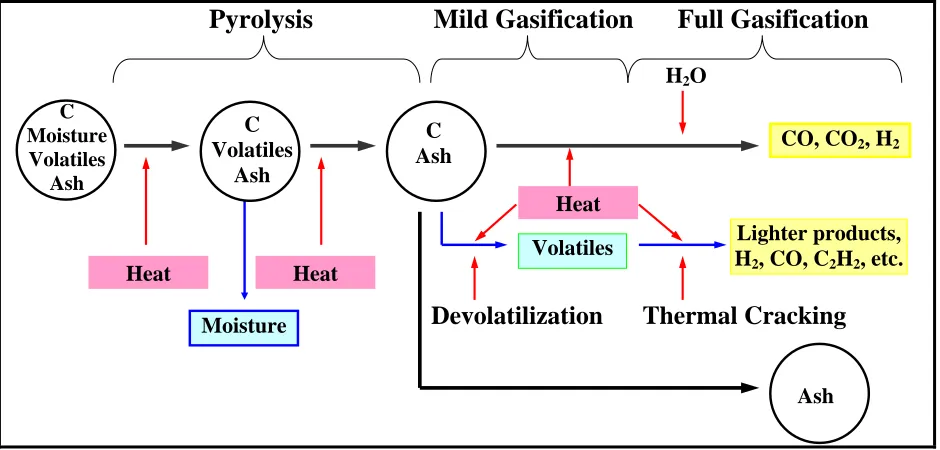
Figure 1.2 presents the typical processes undergone by coal particles in gasification. The gasification of coal particles involves two major steps: (a) thermal decomposition (demoisturization, pyrolysis, and devolatilization) and (b) combustion of solid residue from the first step. Coal particles undergo demoisturization and pyrolysis while facing the hot combustion environment.
The volatiles are then released as the particle temperature continues to increase. The process by which this occurs is called devolatilization. The volatiles are then thermally cracked into lighter gases, such as H2, CO, C2H2, CH4, etc. These lighter gases can further react with O2, releasing some of the heat
needed for the pyrolysis.
With only char and ash left, the particles undergo combustion to produce CO and CO2, leaving
5
C Moisture Volatiles
Ash
C Volatiles
Ash
C Ash
Volatiles Heat
Ash CO, CO2, H2
Heat
H2O
Thermal Cracking
Lighter products, H2, CO, C2H2, etc.
Moisture Devolatilization
Full Gasification
Mild Gasification
Pyrolysis
Heat
Figure 1.2 Simplified global gasification processes of coal particles (sulfur and other minerals are not included in this figure). Heat can be provided externally or internally through combustion of char, volatiles, and CO.
1.2.2.1 Pyrolysis
6
Figure 1.3 Schematic drawing of Pyrolysis of Carbonaceous Fuels
1.2.2.2 Devolatilization
Devolatilization process takes place while hydrocarbon materials are absorbing heat. Temperature, residence time, particle size, and coal type all can influence devolatilization rates. The heating causes chemical bonds to rupture and both the organic and mineral parts of coal to thermally decompose. Such a process starts at a temperature around 100 C (212 F) with desorption of gases, for example, water/steam, CO2, CH4, and N2, which are stored in the coal pores. When the temperature goes
beyond 300 C (572 F), the released liquid hydrocarbon consists primarily of tar. Gaseous hydrocarbons such as CO, CO2, and water/steam are also released. From here, coal particles are in a
plastic state, where they undergo drastic changes in size and shape, while the temperature rises above
500 C (932 F). The coal particles then become hard again, and together are called char, when the
temperature reaches around 550 C (1022 F). As heating continues, H2 and CO are released.
7
coal results in larger particle porosity, while low volatile particles have smaller porosity and burn on the surface.
The pyrolysis conditions affect the physical properties of coal chars. Gale et al. (1995) conducted
an experiment with maximum particle temperatures between 570 C (1058 F) and 1355 C (2471 F) and heating rates between 104 and 2 x 10⁵ K/s, to prove that micro-pore (CO2) surface area generally
increases with increasing residence time and mass releases for lignite and bituminous coals. It also indicated that the micro-pore surface area of char increases with increasing maximum particle temperature and heating rate.
Temperature distribution in the particle depends on volatile matters generated during heating. The volatiles generated near the center of the particle travel to the particle surface and escape. The flow of these volatiles from the particle center to the particle surface can reduce the convective heat transfer from the surroundings to the particles surface. It has been found that the heat transfer coefficient decreases by 10 times during fast heating of coal particles mixed with a hot solid heat carrier. This reduced heat transfer rate to the particle surface results in a temperature plateau of the particle surface on the level of about 400 C (752 F) and lasts during the whole time of volatile release. Davies and Brown (1969) gave another explanation for this temperature plateau is that this is caused by a strong effect of devolatilization.
In general, the larger the particle size, the smaller amount the volatile yields. This is due to the fact that, in larger particles, more volatiles may crack, condense, or polymerize with some carbon deposition occurring during their migration from the inside to the particle surface. High pressure has an identical effect on the devolatilization rates. Anthony et al. (1975) reported that devolatilization rates are higher at lower pressures. An increase in pressure increases the transit time of volatiles to diffuse to particle surface.
8
pressure ranging from 1 to 13 atm with a heating rate as low as 0.33 K/s. It was reported that, at high pressure, the total volatile yield decreases with increasing pressure. The total weight loss is almost independent of pressure at low temperatures (less than 837 K).
Fatemi et al. (1987) studied the pressure effects on devolatilization of pulverized coal with operation temperatures of up to 1373 K and a pressure of 68 atm in an entrained bed reactor. They found that the tar yield decreases significantly with increasing pressure up to 13.8 atm. Weight loss and gas yield both decrease with increasing pressure up to 13.8 atm, but there is no significant effect above this pressure.
Wall et al. (2002) reviewed the pressure effect on variety aspects of coal reactions reported in open literature. In general, the total volatile and tar yields decrease with increasing pressure. This effect is more pronounced at higher temperatures than high pressures. Increasing pressure improves the fluidity of the coal melting and reduces char reactivity.
1.2.2.3 Carbon Particle Combustion/Gasification
The steps involved in a reaction between a gas and a solid particle are as follows:
1. Transport of reactants to solid surface by convection and/or diffusion. 2. Adsorption of reactant molecules on the particle surface.
3. Reaction steps involving various combinations of adsorbed molecules, the surface, and the gas-phase molecules.
4. Desorption of product molecules from the surface.
5. Transport of product molecules away from the solid surface by convection and/or diffusion.
9
surface area reaches a maximum at burnout of about 40%. The total active surface area is then decreased as a result of the interconnection of enlarging neighboring pores.
1.2.3 Particle Combustion Model
(a) Random Pore Model
The random pore model (Bhatia and Perlmutter, 1980) accounts for the evolution of the particle reactive surface during the combustion. The rate of mass change of the particle is defined as follow,
o
po k p
A S m R dt dm
(1.1)
Where mp is the particle mass, mpo is the initial particle mass, Rk is the kinetic rate, and A0 is the initial
particle surface area. S is the instantaneous internal reactive surface area, which is defined as follow,
1 x
ψln 1 x 1 S
S
o
(1.2)
Where So is the initial reactive area, x is the conversion factor, and is the structure parameter for the
particular char/coal type.
(b) Kinetics/Diffusion Fixed-Core Model
The kinetics/diffusion fixed-core model considers the diffusion and kinetic rates of the combustion. The size of the particle during the combustion is assumed to be constant. The particle consumption rate is defined as follow,
0
s d
g p
A
k 1 k
1 P dt
dm
(1.3)
Where mp is the particle mass, Pg is the partial pressure of the gas phase species, A0 is the original
particle surface area, kd is the diffusion rate constant, and ks is the kinetic rate constant.
(c) Shrinking Core Model
10 1 r R k 1 R r k 1 k 1 A P dt dm p p dash 2 p p s d 0 g p (1.4)
Where mp is the particle mass, Pg is the partial pressure of the gas phase species, A0 is the initial particle
surface area, kd is the diffusion rate constant, ks is the kinetics rate constant, kd,ash is the ash diffusion
constant, rp is the instantaneous radius of the particle, and Rp is initial radius of the particle.
1.2.4 Gasification Reactions Summary
Coal gasification occurs when the coal is absorbing energy from a limited amount of oxygen and steam in a gasification reaction chamber. The gasification process is very complicated: however, a simplified list of main global reactions involved in the gasification process can be modeled as follows:
Heterogeneous reactions:
C(s) + ½ O2 → CO HR = -110.5 MJ/kmol (R1.1)
C(s) + CO2 → 2CO HR = +172.0 MJ/kmol (R1.2)
(Gasification, Boudouard reaction)
C(s) + H2O (g) → CO + H2 HR = +131.4 MJ/kmol (R1.3)
(Gasification)
Homogeneous reactions:
CO + ½ O2 → CO2 HR = -283.1 MJ/kmol (R1.4)
CO + H2O (g) → CO2 + H2 HR = -41.0 MJ/kmol (R1.5)
(Water-shift)
The gasification of char by the CO2 and H2O, reactions (R1.2) and (R.1.3), respectively, are endothermic
11
1.2.5 Introduction of Different Gasifiers
There are four main gasifier types: (a) fluidized bed gasifier, (b) entrained flow gasifier, (c) transport gasifier, and (d) moving bed gasifier. Explanations of each type and its examples are presented below. The comparisons of these gasifiers are summarized in Table 1.2.
1.2.5.1 Fluidized Bed Gasifier (FBG)
A fluidized bed gasifier (FBG) employs a similar principle of a conventional combustion fluidized bed, but with only partial oxidant to convert carbonaceous feedstock to produce steam, process heat, chemicals, electric power etc. The functional requirements of the fluidized bed gasifier are to convert efficiently and reliably the carbonaceous fuel into raw reducing gas, ash, char, and possibly raw liquid products by combining carbonaceous fuel with oxidant, steam, and/or an external heat source. For solids transport, aeration and the inert gases, such as nitrogen and recycled product gas also fed to the gasifier.
In a fluidized bed gasifier, air or oxygen is injected upward at the bottom of solid fuel bed, suspending the fuel particles. A schematic of a fluidized bed gasifier is presented in Fig. 1.4. The size (5-10mm) and weight of the particles prevent them from blowing out. The fuel feed rate and the gasifier temperature are lower compared to those of entrained bed gasifiers. The operating temperature of a
fluidized bed gasifier is around 1000 C (1830 F), which is roughly only half of the operating temperature of a coal burner. This lower temperature has several advantages:
Lower NOx emission. The temperature is not hot enough to break apart the nitrogen molecules
and cause the nitrogen atoms to join with oxygen atoms to form NOx.
No slag formation. The temperature is not hot enough to melt ash. It is suitable for coals of any
rank (high or low ash content.)
12
Figure 1.4 Schematic of fluidized bed gasifier (Source: Enggcyclopedia)
Fluidized bed gasifiers require a moderate supply of oxygen and steam. Examples of commercial fluidized bed gasifiers are:
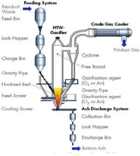
(i) High Temperature Wrinkler (HTW)
The High Temperature Wrinkler (HTW) gasifier was developed by Rheinbraun in Germany to gasify lignite for the production of a reducing gas for refining iron ore. A schematic of an HTW gasifier is presented in Fig. 1.5. The gasifier is a refractory-lined vessel equipped with a water jacket. Coal is dropped into the fluidized bed which consists of particles, semi-coke, and coal. The gasifier is fluidized by the injection of air or oxygen/steam from the bottom. The temperature of the bed is kept at around 800 C (1470 F), which is below the ash fusion temperature. An additional gasification gas is added at the freeboard to decompose undesirable byproducts formed during gasification. The operating pressure can vary from 1 to 3 MPa. The raw syngas exiting the top of gasifier is then passed through a cyclone to remove particulates and then cooled. Particulates recovered in the cyclone are recycled back into the gasifier.
13
no longer considered economically viable. In 1989, a 140 ton/day plant was commissioned in Wesseling, Germany, to supplement research and development of the HTW technology, including the study to future applications for power generation through an Integrated Gasification Combined Cycle system (IGCC). There is presently a project to build a 400 MW IGCC plant in the Czech Republic using the HTW technology developed at the Wesseling plant.
Figure 1.5 Schematic of the High Temperature Wrinkler (HTW) Gasifier (Source: DOE)
(ii) Kellogg-Rust-Westinghouse (KRW)
14
causes the char and the sorbent in the bed to move down the sides of the gasifier and back into the central jet. The char in the bed reacts with the steam, which is injected together with the oxidant and also through multiple other injections on the bottom of the gasifier, to form syngas. The ash particles formed are denser than the coal, thus they settle down to the bottom of the gasifier and are then removed. Any particles that escaped the gasifier through the exit at the top is recaptured in the cyclone gas clean-up system and is then injected back into the gasifier.
In 1997 through 2000, a 965MW Integrated Gasification Combined Cycle (IGCC) demonstration plant using the KRW technology was carried out in Pinon Pine, Nevada, by Sierra Pacific Resources and was sponsored by the U.S. Department of Energy (DOE) as part of its Clean Coal Technology Program. It was the only large-scale coal-based IGCC plant using the KRW technology. Unfortunately, the plant faced numerous problems. It had 18 gasifier start-ups and all of them failed due to equipment design.
15
1.2.5.2 FBG Design Considerations
The design of fluidized bed gasifiers requires developing the transport models of conservation of mass, momentum, and energy. The mass and energy balances are closely coupled and their solutions provide estimates of gas and solids composition, temperature profiles, and input and output stream conditions by applying empirical reaction kinetic and multiple phase mixing models. The momentum balances provide the gasifier pressure profile and total pressure drop by applying appropriate fluidized bed phase density models. The design of fluidized bed gasifiers is related to the selection of several interrelating design, operating, and performance parameters and requires the consideration of performance and cost trade-offs for any specific application. The fluidized bed gasifier is designed to promote a reaction environment having good gas-particle contacting, good particle-particle mixing, and relatively uniform temperature conditions and to avoid operational difficulties resulting from the agglomeration, deposition, erosion, and corrosion of carbonaceous fuels.
1.2.5.3 Fluidization Velocity
A chemical engineering as well as mechanical engineering operation commonly involves the use of fluidized beds. These are devices where a large surface area for contact between a liquid and a gas (absorption, distillation) or a solid and a gas or liquid (adsorption, catalysis) is obtained for achieving rapid mass and heat transfer, and particularly in the case of fluidized beds, catalytic chemical reactions. The theory and empirical correlations associated with thermal-flow fundamentals in a packed bed are reviewed first, followed by the same in a fluidized bed.
1.2.5.3.1 Minimum Fluidization Velocity of Packed Beds
16
ammonia. The soluble species is absorbed in the liquid, and the lean gas leaves the column at the top. The liquid, rich in the soluble species, is taken out at the bottom.
From a fluid dynamics point of view, the most important issue is that of the pressure drop required for the liquid or the gas to flow through the column at a specified flow rate. To calculate this quantity we count on a friction factor correlation dedicated by Ergun. Other fluid dynamics issues involve the proper distribution of the liquid across the cross-section, and developing models of the velocity profile in the liquid film around a piece of packing material so that heat and mass transfer calculations can be made. Design of packing materials to achieve uniform distribution of the fluid across the cross-section throughout the column is an important subject as well. Here, only the pressure drop issue is reviewed.
The Ergun equation that is commonly used is given below,
75 . 1 Re 150 f p
p (1.5)
Here, the friction factor fp for the packed bed, and the particle Reynolds number Rep, are defined
as follows.
1 V D L p f 3 2 s p
p (1.5a)
And
1 V DRep p s (1.5b)
Using the above friction factor fp and the particle Reynolds number Rep relations, the Ergun equation
becomes,
75 . 1 V D 1 150 1 V D L p s f p 3 2 s f p (1.6)17 Δp = Pressure Drop
L = Length of the Bed
p
= Density of the particle
f
= Density of the fluid
µ = Dynamic viscosity of the fluid
Dp = Equivalent spherical diameter of the particle defined by,
p p p A V particle the of area surface particle the of volume
D 6 6
ε = Void fraction of the bed (ε is the ratio of the void volume to the total volume of the bed)
L R density particles particles all of weight L R bed entire of volume particles of volume bed entire of volume bed entire of volume voids volume 2 2
Where, R = inside radius of the column
Vs= Superficial velocity (
A Q
Vs , where Q is the volumetric flow rate of the fluid and A is the
cross-sectional area of the bed, the theoretical velocity of the fluid assuming no particles)
1.2.5.3.2 Minimum Fluidization Velocity of Fluidized Beds
18
in the past. The catalyst is suspended in the fluid by fluidizing a bed of catalytic particles so that intimate contact can be achieved between the particles and the fluid. Nowadays, fluidized beds are used in catalyst regeneration, solid-gas reactors, combustion of coal, roasting of ores, drying, and gas adsorption operations.
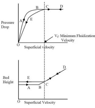
First, consider the behavior of a bed of particles when the upward superficial fluid velocity is gradually increased from zero past the point of fluidization, and back down to zero then calculate the minimum fluidization velocity. The superficial velocity is the velocity of the fluid in the bed if no particles are present.
At first, when there is no flow, the pressure drop is zero, and the bed has a certain height, as shown in Fig. 1.7. The superficial velocity increases along the right arrow, tracing the path ABCD. At first, the pressure drop gradually increases while the bed height remains fixed. When the point B is reached, the bed starts expanding in height while the pressure drop levels off and no longer increases as the superficial velocity is increased. This is happing when the upward force (or upward drag force, Fd)
exerted by the fluid on the particles is sufficient to balance the net weight of the bed (or gravitational force, Fg) and the particles begin to separate from each other and float in the fluid. As the velocity is
19
Figure 1.7 Schematic drawing of Minimum Fluidization Velocity
20
1.2.5.3.3 Calculation of Vmf
One can calculate minimum fluidization velocity, Vmf, by balancing the net weight of the bed
against the upward force exerted on the bed, namely the pressure drop across the bed (∆p) multiplied by the cross-sectional area of the bed (A). Ignoring the small frictional force exerted on the wall of the column by the flowing fluid, the force balance can be formulated as fallows
Upward force on the bed = ∆p A (1.7)
If the height of the bed at this point is "L" and the void fraction is "ε", the volume of particles can be
written as
Volume of particles = (1-ε)AL (1.8)
If the acceleration due to gravity is g, the net gravitational force on the particles (net weight) is
Net Weight of the particles, W
pf
1
ALg (1.9)Balancing the equation 1.5 and equation 1.7 yields the following relation,
g Lp
ALg W
A p
f p
f p
1
1
(1.10)
The various symbols appearing in the above equations are defined as follows. Δp = Pressure Drop
L = Length of the Bed
A = cross-sectional area of the column
p
= Density of the particle
f
= Density of the fluid
21
The point of maximum pressure drop shown in Fig. 1.7 is the point of minimum fluidization. The force balanced equations for the point of minimum fluidization are:
gL p g AL W A p f p mf mf mf f p mf 1 1 (1.11)
According to Ergun equation (Eq. 1.6), the pressure drop increases with the fluid velocity through the following correlation. The first part of the right hand side of Eq. 1.12 is the viscous effect and second part is the inertial effect of fluid.
75 . 1 1 150 1 Re 3 2 N V D L p s f p (1.12)
Where, f s f p Re V D N
= average Reynolds number based upon superficial velocity
Dp = Equivalent spherical diameter of the particle
Vs = Superficial velocity
75 . 1 V D 1 150 1 V D L p s f p f 3 2 s f p (1.13)At minimum fluidization, the superficial velocity, Vs, is equal to the minimum fluidization velocity, Vmf.
At this condition, the above Ergun equation (1.13) is rearranged with Vs being substituted by Vmf, L
substituted by Lmf, and ε substituted by εmf.
22
The minimum fluidization velocity, Vmf, at which fluidization begins can be calculated by combining
Eq. 1.11 and Eq. 1.14 to obtain the following quadratic equations
3
mf mf p 2 mf f 3 mf 2 mf 2 p mf f f p mf 1 D V 75 . 1 1 D V 150 g 1
3mf p 2 mf f 3 mf mf 2 p mf f f p D V 75 . 1 1 D V 150 g (1.15)
2f mf f p 3 mf f mf f p 3 mf mf 2 f 3 p f p
f D 150 1 D V 1.75 D V
g (1.16)
Consider the Archimedes number,
2
f 3 p f p f D g Ar
(1.17)
and the Reynolds number at minimum fluidization,
f mf f p mf V D Re (1.18)
Substituting the Eq. 1.17 and Eq. 1.18 to Eq. 1.16, "Ar" is obtained as,
2mf 3 mf mf 3 mf
mf Re 1.75Re
1 150 Ar
(1.19)
By solving the above quadratic Eq. 1.19 the Reynolds number can be obtained and from Eq. 1.18, the minimum fluidization velocity, Vmf , can be obtained. For large particles (Dp ≥ 1 mm), inertial
effects are important, and the full Ergun Equation, Eq. 1.19, must be used to determine Vmf.
For a bed of small particles (Dp ≤ 0.1 mm), the flow conditions at this stage are such that the
Reynolds number is relatively small (Re ≤ 10) so that the Kozeny-Carman Equation can be used to
23
Ergun equation (Eq. 1.12), which is applicable to viscous flow dominant regimes by removing the inertial part (second part of the right hand side of Eq. 1.12). This yield is given by Eq. 1.20:
mf
3 mf f
2 p f p mf
1 150
D g V
(1.20)
The state of the bed is one of incipient fluidization, when the superficial velocity Vs is equal to
Vmf. The void fraction, ε, at this state depends upon the particle material, shape, and size. For nearly
spherical particles, McCabe, Smith, and Harriott (2001) suggested that ε lies in the range 0.40 to 0.45, increasing a bit with particle size.
1.2.5.3.4 Terminal Setting Velocity
Consider the upward flow of a gas through a bed of particles. At some superficial velocity, the upward drag force (Fd) exerted by the gas on the particles balances the downward body force of gravity
(Fg). This is the condition of minimum fluidization (where, Fd= Fg). For particles with diameters in the
range of 50 to 500 microns and densities in range of 0.2 to 5,000 kg/m3, fluidization usually can be achieved smoothly with increasing gas velocity. As denoted by Geldart (1972), these characteristics embrace the majority of particles encountered in fluidized beds applications. For such particles, gas velocities above the minimum fluidization velocity result in the occurrence of gas bubbles in the bed, wherein some fraction of the gas flows through the suspension of particles as a continuum phase, while the remaining fraction flows as discrete bubbles rising through the suspension. This is the regime commonly called dense bubbling fluidization. The upper limit of the gas velocity for this regime is related to the terminal settling velocity of the particles, beyond which interfacial drag becomes sufficient to entrain the particles out of the bed. To establish the appropriate fluidization regime for any given application, one needs to calculate the minimum fluidization velocity and the terminal settling velocity of the bed particles.
The superficial velocity of the gas for minimum fluidization (Vmf) can be calculated by solving
24
2mf 3 mf mf 3 mf
mf Re 1.75Re
1 150 Ar
Where, the Archimedes number,
2
f 3 p f p f D g Ar
and the particle Reynolds number at minimum fluidization,
f mf f p mf V D Re
When a free-falling object accelerates downwards due to gravity, the upward drag force acting on the object increases, causing the acceleration to decrease. At a particular speed, the downward gravitational force (Fg) will be equal to the upward drag force (Fd). This causes the net force on the object
to be zero, resulting in an acceleration of zero. This particular speed is known as terminal velocity (also called settling velocity).
The terminal velocity (Vts) is given by the expression:
Fd = Fg
D g 6 C D 4 V 2 1 3 p f p D 2 p 2 ts f
D f f p p ts C 3 D g 4 V (1.21)where CD is the drag coefficient for a single particle.
The drag coefficient, CD is equal to 0.44, in the case of spherical particles. But in the case of
near-spherical particles, over the range 1 < Rets < 1,000, CD is given by the relationship:
5 3 ts D 18.5Re
C (1.22)
where the Reynolds number at terminal velocity (Ret) is defined by the following equation:
Fd
25 f ts f p ts V D Re (1.23)
Substituting Eq. 1.22 into Eq. 1.21, an explicit equation for the terminal settling velocity is
Obtained:
7 5 5 3 f 5 2 f f p 5 8 p ts D g 072 . 0 V
Now, consider the condition one must impose on the superficial velocity so that particles are not carried out with the fluid at the exit. This would occur if the superficial velocity is equal to the terminal settling velocity of the particles.
If one’s attention is restricted solely to small particles (Dp ≤ 0.1 mm), Stokes’s Law can then be
used to calculate their terminal settling velocity as:
f 3 p f p ts 18 D g V (1.24)
By using the result for the minimum fluidization velocity for the case of small particles, as in Eq. 1.20, the ratio of Eq. 1.24 and Eq. 1.20 can be found as:
3 mf mf mf ts 1 3 25 V V (1.25)For all "ε" in the range of 0.40 to 0.45, which yields a ratio ranging from 78 to 50.
1.2.5.3.5 Calculation Results of Minimum Fluidization Velocity
26
ambient air, the minimum fluidization velocity needs to be calculated as a reference value for the purpose of simulating coal gasification. The approaches that have been used are given below.
Table 1.2: Properties of the two phases
Properties Gas (air) Particles (carbon solid)
Density, ρ (kg/m3
) 1.225 2000
Heat capacity, cp (kJ/kg K) 1006.43 0.71
Thermal conductivity, k (W/m K) 0.0242 119
Viscosity, µ (kg/m s) 1.7894 x 10⁻⁵ 1.72 x 10⁻⁵
According to Geldart's classification, the carbon solid belongs to type B. The void fraction at the point of minimum fluidization is found to be εmf = 0.60. Assuming the sphericity of the carbon solid to
be Φs = 1.0, the Archimedes number must first be found by solving Eq. 1.17, yield Ar = 2097.40. Then,
the Reynolds number at the minimum fluidization is found by solving the equation Eq. 1.19, and then the value Remf = 6.62 is obtained. From this Reynolds number, the minimum fluidization velocity can be
obtained in terms of solving Eq. 1.18, yielding: Umf = 0.3868 m/s. The following are other equations that
can be used to find out the minimum fluidization velocity of carbon solid that are used in this study.
Todes and Ciovich (1981) suggested:
Ar Ar d U g p g mf 25 . 5 1400 (1.26)
Saxena and Vogel (1977) recommended:
25.282 0.0571 0.525.28
Ar d U g p g mf (1.27)
Finally, Kumer and Gupta (1980) indicated:
78 . 0 005 . 0 Ar d U g p g mf
27
1.2.5.4 Review of FBG History
In 1952, Ergun reviewed and studied the existing information on the flow field through beds of granular solids. In his research work, he described experimental results obtained for the purpose of testing the validity of the various equations and numerous other pieces of data taken from the literature. He found that pressure drops are due to simultaneous kinetic energy and viscous energy losses, and gave the following comprehensive equation for all types of flow.
p 2 m f 3 2 p m f 3 2 D V 1 75 . 1 D V 1 150 L p (1.29)Viscous energy losses per unit length are expressed by the first term of the right hand side of the above equation, and the kinetic energy losses are expressed by the second term of right hand side. Ergun also examined the above equation from the prospective of its dependence upon the fluid flow rate, properties, and fractional void volume (ε) and the orientation, size, shape, and surface of the granular solids.
Whenever possible, conditions were chosen so that the effect of one variable at a time could be considered. A transformation of the general equation points out that the Blake-type friction factor has the following form:
Re 1 150 75 . 1 Nfv
(1.30)
In Ergun’s report, a new concept of friction factor, fv, representing the ratio of pressure drop to the
viscous energy term is discussed as well.
28
to be very useful for explaining heat transfer coefficients from a horizontal tube to a fluidized bed. The Illinois Institute of Technology (IIT) developed a fluidized bed model for a two dimensional bed in cold flow only, which was able to predict void distribution, solids circulation, and bubbling behaviors. Further, this model was extended to a heated fluidized bed. Their results show that, in a bubbling bed, the large heat transfer coefficients can be computed from their hydrodynamic model without the use of any turbulence. This model computes a transient type behavior caused by the formation of bubbles, their propagation, and their eruption at the top of the bed. All of the computed variables including the void fraction, the gas and solid velocities, and the temperatures exhibit a complex oscillatory behavior.
Syamlal (1987) developed a multi-particle model of fluidization phenomena. He simulates fluidization, for example, as segregation, elutriation, and solids mixing. The concept known as particle-particle drag is required for his model as it accounts for the momentum transfer between the particulate phases due to collisions. Earlier researchers developed empirical correlations and measured the particle-particle drag for dilute systems, such as pneumatic conveyors. Similar measurements, however, are not possible to be completed in dense systems, such as a fluidized bed. Therefore, based on the kinetic theory of dense gases, he derived an expression for the particle-particle drag, and then compared the predictions of the model with Yang’s and Keairns’s experimental data in order to test the accuracy of that expression. Yang and Keairns (1982) used uniform mixtures of dolomite and acrylic particles in a fluidized bed many times. They also measured the rate of separation of the dolomite particles from the acrylic particles. They found that the dolomite particles settled rapidly due to it being heavier and larger than the acrylic particles. Yang and Keairns's experimental data suggest that the rate of settling is strongly dependent upon the particle-particle drag. Therefore, for determining the accuracy of the equation for particle-particle drag, duplicating Yang and Keairns experiments is a necessary endeavor. He found that the model predicts the initial rate of separation reasonably well. But, the predicted equilibrium concentrations of dolomite particles in the upper layer of acrylic particles do not agree with the experimental data. He thought this is because of the absence of granular stress from the model. Hence, further refinement of the particle-particle drag term can be sought only after including realistic granular stress in the multi-particle model.
29
fluidized beds of various particle sizes, with and without jets can also be modeled. They found that the predicted characteristics of bubble formation, bubble motion, bubble eruption at the surface, bubble shape, bubble coalescence phenomena, and also the dynamics of the bed surface are in good qualitative agreement with experimental data. They compared the bubble volume, bubble rise velocities, bubble frequency, wake angle, wake fraction, and pressure profile with experimental data and simpler theories. They tested the predicted gas and solids mixing by using a new graphical technique and found that the data is in good agreement with experimental results.
Benyahia et al. (2004) investigated the capability of three gas-solid flow models (standard granular kinetic theory and two gas-solid turbulence models) to estimate the core-annular flow behavior usually observed in dense gas/solid flows. Their study proved that the granular kinetic theory, Balzer et al. 1996, and Cao and Ahmadi 1995 give similar estimation of a dense, fully-developed flow in a vertical channel and that the gas turbulence may not have a dominant effect in relatively dense gas/solid flows. Eventually, the core-annular flow behavior in which the maximum concentration of solids occurred at the walls was not observed if the boundary conditions cause production of granular energy at the wall. Boundary conditions that dissipate granular energy near the wall are needed to induce a core-annular flow structure.
Gunn (1978) experimentally measured the heat transfer to and from particles in fixed beds and showed that either the Nusselt number decreases to zero if axial dispersion has been neglected, or the Nusselt number remains at a constant value as the Reynolds number is reduced. A quantitative analysis of particle to fluid heat transfer upon a stochastic model of the fixed bed leads to a constant value of the Nusselt group at low Reynolds number. When the analytical equation contains an asymptotic condition, he derived an expression which describes the dependence of the Nusselt group upon Reynolds number. In addition, he extended this expression to describe mass and heat transfer to fixed and fluidized beds of particles within the porosity range of 0.35 to 1.0. Both the gas and liquid phase transfer groups were correlated up to a Reynolds number of 105.
30
coefficients of restitution (inelastic particles) and a second for the general flow of particles with coefficients of restitution near one (slightly inelastic particles). The study of inelastic particles in Couette flow duplicated the method of Savage & Jeffrey (1981). An ad hoc distribution function was used to simulate the collisions between particles. They compared the results of this first analysis with other theories of granular flow, with the Chapman-Enskog dense-gas theory, and with experiments. Their theory agreed moderately well with experimental data, and it is found that the asymptotic analysis of Jenkins & Savage (1983), which was developed for slightly inelastic particles, gave wonderful results that are similar to the first theory even for highly inelastic particles. Thus, the "nearly elastic" approximation is pursued as a second theory using an approach that is closer to the established methods of the Chapman-Enskog dense-gas theory. By defining the collisional distribution functions through a rational approximation scheme, their new approach is not only applicable to normal flow fields, but to simple shear flows as well. It incorporates kinetic as well as collisional contributions to the constitutive equations for stress and energy flux and is thus appropriate for dilute as well as dense concentrations of solids. While the collisional contributions are dominant, it predicts stresses similar to the first analysis for the simple shear case.
Ding and Gidaspow (1990) indicated that, for a better understanding of tube erosion in fluidized bed combustors, detailed knowledge of bubble motion, solid circulation, and the frequencies of porosity oscillations is required. They suggested a predictive two-phase flow model starting with the Boltzmann equation for the velocity distribution of the particles. This model is a generalization of the Navier-Stokes equations of the type proposed by R. Jackson, except that the solid viscosities and stresses are computed by simultaneously solving a fluctuating energy equation for the particulate phase. Predictions from this model agree with the time-averaged and instantaneous porosities measured in two-dimensional fluidized beds. They also estimated the bubbles and observed flow patterns.
31
incorporation of turbulence terms in the transport equation. Their calculation clearly showed the enhancement of the wall-to-bed heat transfer process due to the bubble-induced bed-material refreshment along the heated wall. The model proved its usefulness and distinguished itself advantageously from former theoretical models by offering detailed information on the local behavior of the wall-to-bed heat transfer coefficients. The local wall-to-bed heat transfer coefficient is relatively large in the wake of the bubbles rising along the heated wall because of the vigorous solid circulation in the bubble wake.
Enwald et al. (1999) investigated a validation of the two-fluid model for a bubbling fluidized bed application and a mesh refinement study for the same. They calculated the simulated statistical bubble quantities from voidage signals derived from the transient multidimensional solution of two-fluid models. The algorithm for computing these quantities was taken directly from the evaluation program treating the measurement signals. They developed a parallel version of the two-fluid model solver to remedy the long simulation times required to obtain acceptable statistical values. This version was based on a domain decomposition method for distributed memory computers. The mesh refinement study indicates that a higher degree of mesh refinement is required for atmospheric than for pressurized fluidization. They evaluated statistical bubble parameters (bubble frequency, mean bubble rise velocity, mean pierced bubble length, and mean bubble volume fraction). They investigated a number of problems related to the parallelization. These problems are related to the optimal treatment of the velocity components with respect to the frequency of data exchange at multi-block boundaries, local errors at multi-block boundaries, and simulation time requirements.