Imaging unresolved object using vortex mode detection

(1)

Rochester Institute of Technology

RIT Scholar Works

Theses Thesis/Dissertation Collections

3-16-2012

Imaging unresolved object using vortex mode

detection

Jiaxuan Han

Follow this and additional works at:http://scholarworks.rit.edu/theses

This Thesis is brought to you for free and open access by the Thesis/Dissertation Collections at RIT Scholar Works. It has been accepted for inclusion in Theses by an authorized administrator of RIT Scholar Works. For more information, please [email protected].

Recommended Citation

(2)

RIT

Imaging Unresolved Object using Vortex Mode Detection

by

Jiaxuan Han

A thesis submitted in partial fulfillment of the requirements for the degree of Master of Science in Imaging Science in the Chester F. Carlson Center for Imaging Science,

Rochester Institute of Technology.

Chester F. Carlson Center for Imaging Science College of Science

Rochester Institute of Technology Rochester, NY

March 16, 2012

Committee Approval:

Grover Swartzlander Date

Advisor

Zoran Ninkov Date

Committee Member

Mishkatul Bhattacharya Date

(3)

Abstract

Resolution is an imaging system's ability to distinguish object detail. The resolution

ability is ultimately limited by diffraction, which is hard to avoid because it comes from

the wave nature of light. The Rayleigh criterion given by the finite width of the Airy

disk, is the generally accepted criterion for the minimum resolvable detail. This

criterion was hard to overcome until the study of Optical Vortex Coronagraph (OVC) system. This system can eliminate the component of light that creates Airy disk. The

left light, which can pass through the OVC system, contains spatial information from

the observed object even if it is an unresolved object as defined by the Rayleigh

criterion.

This thesis challenges the Rayleigh criterion using the OVC system. It is not hard to

obtain the feature information of a object by detecting the light power that enters the

system and the power that eventually passes through the system. A binary points source

example in this thesis shows that, even if the source is unresolved under the Rayleigh

criterion, its power transmission contains the information of angular extent of the two points sources. The power transmission of an ellipse object can differentiate tiny

(4)

Acknowledgements

My graduate study in the Center for Imaging Science includes some of the most fun and

valuable times in my life. I am very happy to the opportunity to learn imaging-related

knowledge and skills with the help and encouragement of many people.

First, I would like to thank my advisor, Dr. Grover Swartzlander, for his careful guidance and inspiring advice. He taught me the skills I needed to complete my M.S.

Degree. Thanks also go to my committee member, Dr. Mishkatul Bhattacharya and Dr.

Zoran Ninkov.

I would also like to thank my parents for their care and support. I could not come to

(5)

3. Examples...32

3.1 Single point source...32

3.2 Binary point source...35

3.3 Ellipse source...46

3.4 Summary...54

4.

Summary and Future work...56

4.1 Summary...56

(6)

Appendix...58

A. The first kind Bessel function...58

B. Related integral of Bessel function...59

(7)

LIST OF FIGURES

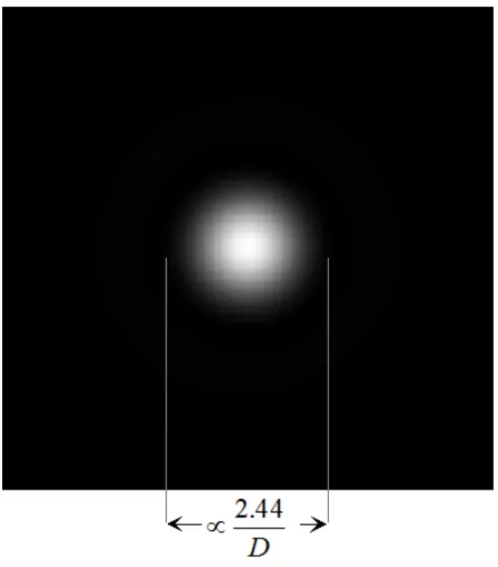
Fig. 1.1 Image of the point source produced by Fraunhofer diffraction. The size of the Airy disk is proportional with 2.44/D. (D is the diameter of the aperture)...3

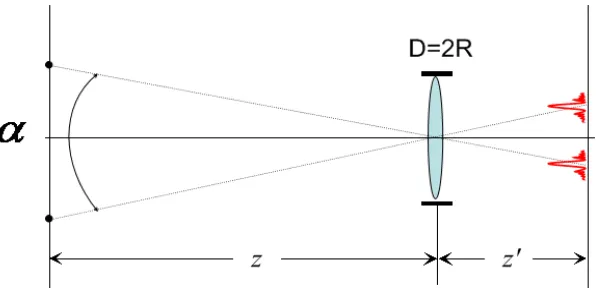
Fig. 1.2 Image system, includes two point sources separated by α, a lens located far away from sources marked z, the image of two sources are produced by Fraunhofer diffraction...4

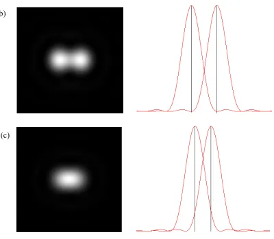
Fig. 1.3 Image of two point sources with different separation. (a) These two stars are clearly resolvable, as their Airy disks do not overlap. (b) These two stars are just resolvable although the Airy disks overlap, they are separated by more than the Airy disk radius.(c) These two stars are not resolvable...5

Fig. 1.4 Optical vortex coronagraph with aperture stop, vortex lens, imaging lenses, Lyot stop, and camera...6

Fig. 1.5 Helicoid wave front (with vortex charge m=2)...7

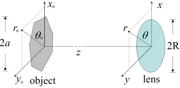
Fig. 2.1 An object of extent 2a radiates light of wavelength λ to the far field region

(z>> πa2/λ) where it is collected by a lens with diameter 2R...11 Fig. 2.2 Normalized amplitude profile of the modesG_l2_,_n(r'',θ '')at the Lyot Stop. Vortex charge m=2...22

Fig. 2.3 Normalized amplitude profile of the modesG_l4_,_n(r'',θ '')at the Lyot stop. Vortex charge m=4...26

Fig. 2.4 Normalized amplitude profile of the modesG_l6_,_n(r'',θ '')at the Lyot stop. Vortex charge m=6...29

Fig.3.1 Image at the aperture of a single point source ( With πa/λz=0.5 and θI =45

degree)...33

(8)

telescople...36

Fig. 3.2a Image of coherent binary point source at the Lyot stop, with vortex charge

m=2, and γ<1...38

Fig. 3.2b Image of coherent binary point source at the Lyot stop, with vortex charge

m=4, and γ<1...39

Fig. 3.2c Image of coherent binary point source at the Lyot stop, with vortex charge

m=6, and γ<1...39

Fig. 3.3a Image of incoherent binary point source at the Lyot stop, with vortex charge

m=2, and γ<1...40

Fig. 3.3b Image of incoherent binary point source at the Lyot stop, with vortex charge

m=4, and γ<1...40

Fig. 3.3c Image of incoherent binary point source at the Lyot stop, with vortex charge

m=6, and γ<1...41

Fig 3.4 Compare binary points source power transmissions with different non-zero vortex charge m when the source is coherent and incoherent...44

Fig.3.5 Calculation for Bl when object is a ellipse with radius a and b. There are three situations for calculation of Bl : ro<b, b<ro<a and ro>a...45 Fig. 3.6 The image of ellipse source at the aperture of telescope. (The ratio of long radius and short radius of ellipse source is a/b=2,and πRb/(λz)=0.7)...48

Fig. 3.7 Image of ellipse source at the Lyot stop, with vortex charge m=2, and

πRa/λz<1...49

πRa/λz<1...50

(9)

Fig.3.10 For the ellipse object, power transmission ηm varies with ratio of the object radius t=a/b when assume πRb/(λz) is constant...52

Fig.3.11 For the ellipse object, power transmission ηm varies with the extent of the object γ=πRb/(λz), assume ratio of the object radius t=a/b is constant...53

Fig.A.1 Graphs of the first kind Bessel function Jα(x), α=0,1,2,3...58

(10)

1 Background

Resolution quantifies the ability of an imaging system to be able to differentiate one object from the other found within the same field of view. The imaging system's

resolution is always limited by aberration and diffraction effects. Aberration, in

principle, can be solved by increasing the system's optical quality. However, for the

finite aperture of an optical element and the wave nature of light, the diffraction effect

is hard to avoid. A well known criterion chosen by Lord Rayleigh to define the limit of resolution of a diffraction-limited optical instrument is the Rayleigh criterion. It is

the condition that arises when the center of one diffraction pattern is superimposed

with the first minimum of another diffraction pattern, produced by a point source

equally bright as the first. By this criterion, two adjacent objects cannot be resolved if

the profiles of the two diffracted images are not far enough separated.

This thesis will take a different approach to overcome this criterion. The optical

vortex coronagraph (OVC) system, which is built up with aperture stop, vortex lens,

imaging lenses, Lyot stop and detector, can capture the features information exists in

the detectable vortex modes, although an object may have unresolvable features. Such vortex modes are described by circular harmonic decomposition components and can

be applied to all objects. This chapter will introduce more details about the Rayleigh

criterion and the OVC system.

(11)

1.1 Rayleigh Criterion

The Rayleigh criterion is a generally accepted criterion for the diffraction-limited

optical instrument. Consider the image if the object is a point source, such as a star,

observed through a telescope with a circular aperture. The image of the point source is produced by the Fraunhofer diffraction of light by the aperture. The resulting

irradiance produced by the point source at the image plane is,

2 1

sin ) sin ( 2 ) 0 ( ) (

  

 =

θ θ θ

kR kR J I

I (1.1)

where I(0) is the peak irradiance at the centre of the diffraction pattern, R is the radius

of the aperture, k is the wave number 2π/λ and J1(x) is the first order Bessel function (Appendix A), and θ is the angle of observation (i.e. the angle between the axis of the circular aperture and the line between aperture center and observation point).

The central region of the profile, from the peak to the first minimum, is called the

Airy disk. The approximate formula of the angle from the direction of incoming light

to the first minimum is expressed by:

λ θ 1.22 sin

2R _R ≈ (1.2)

where θR is the angular resolution in radians, λ is the wavelength of light. 1.22 is approximately the first zero point of the Bessel function of the first kind, of order one

J1, divided by π. For small angles, we can simply sinθ=θ. Fig.1.1 shows the Frauhofer diffraction of single point source. The diameter of the Airy disk is proportional to 2.44

(12)

[image:12.595.190.414.77.332.2]

Fig. 1.1 Image of the point source produced by Fraunhofer diffraction. The size of the Airy disk

is proportional with 2.44/D. (D is the diameter of the aperture)

If we have two point sources extremely close together, their Airy disks will overlap. According to the Rayleigh criterion, it is only possible to resolve a pair of sources if

the central peaks of the two diffraction patterns are no closer than the radius of the

Airy disk.

Fig.1.2 plots a general imaging system with a lens and a circular aperture. Two

(13)

[image:13.595.151.449.76.227.2]

Fig. 1.2 Image system, includes two point sources separated by α, a lens located far away from

sources marked z, the image of two sources are produced by Fraunhofer diffraction.

Two point sources are regarded as just resolved when the principal diffraction

maximum of one image coincides with the first minimum of the other (the distance between central peaks of the two diffraction patterns is equal to the radius of the Airy

disk). If the distance is greater, the two points are well resolved; if it is smaller, the

(14)

[image:14.595.100.500.77.427.2]

Fig. 1.3 Image of two point sources with different separation. (a) These two stars are clearly

resolvable, as their Airy disks do not overlap. (b) These two stars are just resolvable - although the

Airy disks overlap, they are separated by more than the Airy disk radius. (c) These two stars are

not resolvable.

(15)

1.2 Vortex coronagraph architecture

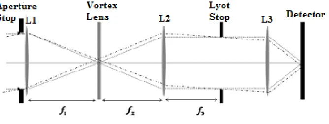
The optical vortex coronagraph[1],[2],[3] (depicted in Fig.1.4) is arranged with an

aperture stop, vortex lens, imaging lenses, Lyot stop, and detector. Light from a

distant object is imaged by L1, which represents telescope optics. A vortex lens is placed near the back focal plane of the objective lens L1. Lens L2 collimates the light

after the light passes through the vortex mask. The front focal plane of L2 is near the

back focal plane of L1. Between L2 and L3, a circular Lyot stop blocks unwanted

light thereby allowing the enhanced detection of nearby objects. The remaining light

[image:15.595.137.471.411.537.2]

is then re-imaged by L3. When the vortex mask is absent, an image of the pupil by lens L2 appears in this exit pupil plane.

Fig. 1.4 Optical vortex coronagraph with aperture stop, vortex lens, imaging lenses, Lyot stop, and

camera.

Not all light which emitted from the observed object entering the aperture can pass

through the Lyot stop, part of the light will be diffracted outside the Lyot stop. The

most dominant component among the eliminating light is a plane wave component

which does not make a contribution to resolving the object. The remaining

(16)

shape of the source object. Although an object may have unresolvable features, the

detectable light may still show such information about the object. By this way, it is

possible to overcome the Rayleigh criterion using the OVC system (calculation will

be shown in the second chapter).

1.3 Vortex Lens

An important element in the design of the OVC systems is the Vortex lens, which is

also called phase mask. The Vortex lens can transform a planar wave front into a

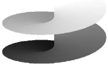
[image:16.595.204.392.402.517.2]

helicoid wave (as Fig. 1.5).

Fig. 1.5 Helicoid wave front (with vortex charge m=2)

Writing the incident plane wave as E0(r,θ), after it transmits through a vortex lens,

the field will be expressed as[4]

) , ( ) ( ) ,

(r θ t θ E₀ r θ

E = _m (1.3)

where tm(θ)=exp(imθ) is the vortex lens transmission function; r and θ are circular coordinates; m is called vortex charge, which characterizes the beam's helical

(17)

winding around the optical axis.

A surface with the ideal transmission function tm(θ)=exp(imθ) is hard to produce in a real production process. Instead of continuous surface, a good quality vortex lens is

always produced with binary structures, having discrete step heights. The corresponding transmission function can be expressed as a Fourier series of vortex

modes of order l:

∑

∞

−∞ =

=

l

l il C

t(θ) exp( θ) (1.4)

where = −

∫

−

π

θ θ θ

π 2

0 1

) exp( ) ( ) 2

( t il d

C_l is the Fourier series coefficient. Therefore, for

producing an N-level vortex lens with topological charge m, the discrete transmission function may be written as tj=exp(iΦ_j), where Φ_j =2πmj/N for j=0,1,...,N-1. Thus, the Fourier series coefficients are given by

) ( ,

) / exp( ) / (

sin _l _m _kN

l c l N il N

C = π − π δ ₊ (1.5)

where δ_l_,₍_m₊_kN₎ is the delta function, and k is an integer. Due to the spectrum of the vortices produced by discrete, regularly spaced phase level does not produce vortices at all values of l, but rather, at the values l=m,m±N,m±2N,m±3N,...

For each discrete pitch, its maximum height is related to the design wavelength λ, desired topological charge m, and refractive indexes of the substrate and the surrounding material. An equation about the relationship between these factors

is[4]

(

)

0 0

/µ _λ

λ n n m

d = _s−

(18)

design wavelength.

1.4 Summary

In the traditional method, the limit of resolution of a diffraction-limited optical

instrument is the Rayleigh Criterion, which is related to the size of the Airy disk. However, it is possible to overcome the limit of the Rayleigh Criterion, if avoid

detecting the Airy disk. The OVC system may realize it. Compared with the

traditional coronagraph system, the OVC system has an additional instrument, the

Vortex Lens, which can transform a planar wave front into a helicoid wave and leads

(19)

2. Methodology

This chapter will analyse the method of detecting unresolved object using OVC in principle.

This thesis only examines the extremely paraxial rays. Assume the telescope is

located far away from the observed object, then the field at the telescope's aperture

can be described as the Fraunhofer diffraction. Mathematically, the Fraunhofer diffraction is proportional to the Fourier transform of the object distribution. When

the object can be expressed as the circular function, the Hankel transform can depict

this Fourier transform. After the light from the object passes through the vortex

coronagraph, certain components may be diffracted outside the Lyot stop and will not be detected by the camera. Such as when the vortex charge m≠0, the plane wave

component (l=0) will be diffracted outside the Lyot stop, which is the most dominant

component but not useful to discern the position and shape of the observed object.

However, the remaining components always contains the feature information of the

source.

2.1 Circular Harmonic Decomposition

In the polar coordinate, functions that represent physical situations are periodic with

period 2π. When the object function f (xo,yo) is written as f (ro, θο), its decomposition

would be[7],[8],[9]

∑

∞

−∞ =

=

l

o o

l o

o B r il

r

(20)

The sum is understood to be from −∞to+∞, and the Fourier coefficient Bl is given

by

∫

−

= π θ θ

π

2

0

) exp( ) , ( 2

1 )

(_o _o _o _o _o

l r f x y il d

B (2.2)

The point (ro,θo) represents circular coordinates in the xo,yo-plane. The intersection of the plane with the optical axis of the imaging system is ro=0. Thus, the object function

always can be expressed as the sum of the Fourier series in the polar-coordinate

system.

2.2 Object Source Propagates to The Telescope

Define the plane where the object f(xo,yo) located as the xo-yo plane and specified by

z=0. As shown in Fig.2.1, the telescope observed the electronic field radiated by the

object at an observation plane z>>0, named x-y plane, and it is the place where the

telescope's aperture located.

[image:20.595.151.456.548.697.2]

(21)

The Fraunhofer diffraction, which describes the light transform when the

observation plane located a large distance, is proportional to the Fourier transform of

the object distribution[10]. The restriction of the Fraunhofer diffraction is that the

object and observation points are sufficiently close to the axis, meansx_o2+y_o2<<λzandx2+y2 <<λz(where λ is wave length of light). According to the Fraunhofer diffraction, the field at the observation plane is expressed as:

(

)

)} , ( { ] 2 exp[ 1

)] (

2 exp[ ,

)] (

exp[ ] 2 exp[ 1 ) , (

2 2

z y z x f FT z i z

i

dy dx y y x x z

i y

x f

z y x i z i z

i y x E

o o o o o

o

λ λ λ

π λ

λ π λ π λ

π λ

⋅ =

+ −

⋅

+ ≈

∫ ∫

∞ +

∞ −

∞ +

∞

− (2.3)

where FT stands for the Fourier transform, and the large value of z ensures that the

leading quadratic phase term is approximately unity and may be neglected. One thing

needs to note here is that both the object pattern f(xo,yo) and the pattern in observation

plane E(x,y) are in the space domain, Fourier transform is a tool to relate the

distribution in these two planes.

2.3 Hankel Transform

When the function f(x,y) can be expressed as a separable form f(x,y)=fr(r)exp(ilθ), its

Fourier transform may be written as the Hankel transform. The subscript r is used to

(22)

∫ ∫

∞ + ∞ − + − +∞ ∞ − + − = = dxdy e il r f dxdy e y x f y x f FT y x i r y x i ) ( 2 ) ( 2 ) exp( ) ( ) , ( )} , ( { η ε π η ε π

θ (2.4)

Where ε and η correspond to spacial frequence,and the 2D Fourier mask function

e-2π i(εx+ηy) can be recast into polar coordinates,

]] cos[ 2 exp[ ])] sin[ ] sin[ ] cos[ ] cos[ ( 2 exp[ ) ( 2 φ θ ρ π φ ρ θ φ ρ θ π η ε π − − = + − = + − ir r r i

e i x y

(2.5)

where ρ corresponds to spacial frequency, and φ corresponds to angular spacial frequency.

The differential element of the area must covert to rdrdθ polar representation. The domain of integration of the radial variable in polar coordinates is 0≤r<+∞, while

the azimuthal variable must cover a full circle of 2π. Therefore, the polar form of the 2D Fourier transform is

∫

+∞ − − = 0 2 0 )) cos( ( 2 ) ) exp( )( ( )} , (

{f x y f r il e d rdr

FT _r θ i r θ

π

φ θ ρ

π _(2.6)

By changing the variable of this integration to ψ=θ−φand using the fact that the cos function is periodic over 2π radian, the azimuthal integral may be rewritten as

) 2 ( ) exp( ) ( 2 ) exp( ) exp( 2 0 ) cos ( 2 2 0 )) cos( ( 2 ρ π φ π ψ φ θ

θ π ψ π ρ ψ

π φ θ ρ π r J il i d e e il d e il l l r i il r i = =

∫

− − − (2.7)

where Jl(z) is the an l-th order Bessel function of the first kind with argument z.

(23)

)} ( { ) exp( ) ( 2

) 2 ( ) ( ) exp( ) ( 2 )} , ( {

0

r f HT il i

rdr r J r f il i

y x f FT

r l l

l r l

φ π

ρ π φ

π

=

= +∞

∫

(2.8)

where HTl is l-th order Hankel transform.

In a word, the 2D Fourier transform of the function, which can be written as the

product of the radial part fr(r) and azimuthal part exp(ilθ), can be expressed as the l-th

order Hankel transform.

2.4 The Field at The Aperture

As discussed above, the distribution of the object can be expressed as a series of

circular harmonic functions. The light field at the observation lens is the Frauhofer

diffraction, whose mathematics expression is the Fourier transform of the object

distribution. The field radiated by the observed source collected by the telescope is the

Hankel transform of the object. By applying Eq.(2.1) and Eq.(2.8) into Eq.(2.3), for the l-th circular componentB_l(r_o)exp(ilθ_o), its corresponding field at the observation

lens El(r,θ) is written as:

( )

{

}

(

/

)

( )

{

( ( )

}

exp( ) )

, ( )

,

( 1

θ θ

λ θ

il r

B HT i z k

r f FT z r

E

o l l l

o o l l

− =

= −

(2.9)

where k=2π /λ, kr = (2π/λ)(ro/z) and

{

} ∫

=∞ 0

) ( ) ( )

( _o _l _o _l _r _o _o _o l

l B r B r J k r rdr

HT (2.10)

(24)

<<1), may be written as[2],

(

)

∑

∞

(

)

= 

   

  

+ + Γ − =

0

2

) 1 (

!

2 / 2

/ )

(

n

n o r l

o r o r l

n l n

r k r

k r k

J (2.11)

If the far-field electric field is collected through an aperture of radius R that satisfies the

extreme paraxial condition, e.g., if the angular extent of the object is much smaller than the

resolution angle of the imaging system (λ/2a), then the sub-resolution criterion may be

expressed:

(2π/λ)(R/z)a << 1 (2.12)

Therefore, the field collected by the instrument (r< R) is approximated by

∑ ∑

+∞ −∞ =

+ ∞

=

l

n l n

n

l r R il

C r

E( , ) ( / ) 2 exp( )

0

, θ

θ (2.13)

Where Cl,n is a constant that depends on the irradiate distribution of the source.

( )

∫

+ +

+

+ + Γ

− −

= a l n _o

o o l n l l

n n

l B r r dr

z z R n

l n

i C

0

1 2 2

, ( )

) / ( ) 1 (

!

) ( 2 1

λ λ π π

(2.14)

Thus, the field at the telescope's aperture plane can be written by a series of modes. Each mode is expressed as C_l_,_n(r/R)|l|+2neilθ.The intensity colleted by the detector,

therefore, can be expressed as the integral of field expression's square. For example, the passing through energy for mode (0, 0) isπR2C₀2_,₀.

Note that, the value of the constant C0,0 is proportional to the area of the

objectaccording to Eq.(2.2) and Eq.(2.14), which means this mode brings no details

(25)

Every object's field at the telescope's aperture can be written as the sum of a series

of circular components

∑ ∑

+∞

−∞ =

+ ∞

= l

n l n

n

l r R il

C ( / ) 2 exp( )

0

, θ . For different sources, their

corresponding components have different constant coefficient Cl,n, but their variables

expression (r/R)l+2nexp(ilθ) are same.

2.5 Light Pass Through The OVC system

The OVC system is arranged with the vortex lens placed in the back focal plane of the

telescope lens[2], as illustrated in Fig.1.4. A Lyot stop is placed in the exit pupil (where the entrance aperture is imaged) to prevent the diffracted light from the object from

reaching the detector. The vortex lens has a negligible effect on light from off-axis

light sources, which transmits through the Lyot stop.

The lens L1 with the focal length f1 located closely after the aperture, which is used

for focusing the light in the focal plane. Ignore the thickness of the lens, its optical

transmission function is[10]:

] exp[

) (

1 2

f r i r

t

λ π

−

= (2.15)

which means that the phase of the transmitted light increases with increasing radial

distance from the optical axis.

The amplitude at the back of the lens L1 is identical to that in the aperture

(26)

) ( ] exp[ ) exp( ) / ( ) , ( ' 1 2 2 0

, P r

f r i il R r C r E l n l n n

l θ π _λ

θ _ −

     =

∑ ∑

+∞ −∞ = + ∞ = (2.16)

For each circular component mode, the field is written as,

) ( ] exp[ ) exp( ) / ( ) , ( ' 1 2 2 ,

, P r

f r i il R r C r

E_l_n _l_n l n

λ π θ

θ = + − (2.17)

P(r) is the pupil function describes the aperture. Assume the aperture has a uniform

transmission, when r is smaller than the radius of aperture R, P(r)=1, else P(r)=0. Because the focal length of the lens in the OVC is relatively small when compared it

with distance z, the Fresnel diffraction can well describe the propagation of the field

from the lens to the corresponding image which can be expressed as a phase term

times the product of two terms' convolution. Define the focal plane of the first lens L1

as x'y'-plane, the light filed at this plane therefore is expressed as:

1 ' , 1 ' 1 2 2 1 1 2 1 1 1 1 1 2 2 1 1 2 1 2 2 1 2 1 1 2 2 )} , ( ) , ( { ] 2 exp[ 1 ) , ( )} , ( { ] 2 exp[ 1 1 ) , ( )} , ( { ] 2 exp[ 1 ) ' , ' ( f y f x f y x i f y x i f y x i f i f y x i y x E y x P FT e f z i zf y f z x f z f f y f x P FT e f z i zf e e f i e y x P z y z x f FT z i z i r g λ η λ ε λ π λ π λ π λ π λ π λ π λ λ λ λ π λ λ λ λ λ π λ θ = = + + + + + + + − ⋅ + − =       − − ∗ + − =           ∗           ⋅ ⋅ = (2.18)

This field is equivalent with a coefficient times two phase terms and Fourier

transform of field distribution at the aperture stop. In order to make the following

calculation more convenient, ignore the coefficient -1/λ2zf1 and phase term

(27)

field in the first lens's focal plane can be simply written as

(

)

(

r R

)

J k r rdr e C i r P e R r C FT r g R r l p il n l l il p n l n l ) ( / ) ( 2 )} ( / { ) ' , ' ( 0 ' ' , , ,

∫

− = = θ θ π θ (2.19)

where kr'=2πr'/λf1, p=|l|+2n.

The vortex lens is in the focal plane modifies the fields to create the distribution,g_l_,_n(r',θ')exp(imθ') by Eq.(1.3).

Then, the beam undergoes another Fresnel diffraction when it propagates to the

plane of the Lyot stop. Define the plane of the Lyot stop as x''y''-plane,where the field

is:

(

)

∫ ∫

∞ + + +         − = = 0 '' 0 ' '' ) ( , 2 2 , ' , ' ' ) '' ( ) ( / ) ( ) 2 ( )} ' , ' ( { ) '' , '' ( dr r r k J rdr r k J R r e C i r g e FT r G r m l R r l p m l i n l m l n l im m n l θ θ π θ θ (2.20)

where kr''=2πr''/λf2.

Finally, after pass through the coronagraph system, the azimuthal expression of the l-th mode is ei(l+m)θ'' , m is the vortex charge. The sum of mode components

∑ ∑

+∞ −∞ = +∞ = = l n m n l m r G r G 0 , ( '', '') ) '' , ' '

( θ θ is net field at the Lyot stop.

2.6 Calculation Samples for Certain Mode's Field at the Lyot Stop Plane

(28)

many lowest modes (l =0,±1,±2Λ ,n=0,1,2Λ ) is sufficient to describe the object's

features. This part will calculate five lowest modes' field at the Lyot stop plane with

three different nonzero value vortex charge m. As discussed above, each mode can be written as Cl,n (r/R)peilθ (p=|l|+2n). The value of Cl,n relates to the object. More

details about the calculation of Cl,n will be shown in the next chapter. This part will

focus on the transform of the variable part rpeilθ..

Assume that the two lenses have the same focal length, ie. f1=f2, and the Lyot stop

has a same size with the aperture in order to make calculation more convenient. If the

vortex charge m=2, by Eq.(2.20) the field of the first mode 1 (l=n=0) at the Lyot stop plane can be written as

( )

   

> −

< =

− =

   

  −

= =

∫

∫ ∫

∫

∞ ∞

R r r

R e

R r

dr r k

r k J R k RJ e

dr r r k J rdr r k J e

i

rdr r k J e FT r

G

i

r r r

i

r R

r i

R r i

'' , ''

'' , 0

' ' ) ' ( ) ( )

2 (

' ' ) ' ( )

( )

2 (

} ) ( {

2 ) ' ' , '' (

2 2 '' 2

0

' '' 2 ' 1 '' 2 2

0

'' 2 0

' 0 '' 2 2 2

0 ' 0 ' 2 2

0 , 0

θ θ

π π π θ

(2.21)

This mode transforms into a ring of fire as illustrated in Fig.2.2, when m=2. Assume

the radius of the Lyot stop is R (same with the aperture size), this mode can not pass

the Lyot stop completely.

(29)

    > < = =       = − =

∫

∫ ∫

∫

∞ ∞ R r r R e R r dr r k r k J R k J R e dr r r k J rdr r k rJ e rdr r k rJ e e FT i r G i r r r i r R r i R r i i , ' ' , 0 ' ' ) ' ( ) ( ) 2 ( ' ' ) ' ( ) ( ) 2 ( } ) ( { ) ( 2 ) ' ' , '' ( 3 4 '' 3 0 ' '' 3 ' 2 2 '' 3 2 0 '' 3 0 ' 1 '' 3 2 0 ' 1 ' ' 2 2 0 , 1 θ θ θ θ θ π π π θ (2.22)

This mode is diffracted outside the Lyot stop entirely too, so there is no information of this circular component can be got at the detector.

When the vortex charge m=2, the field of the modere−iθ at the Lyot stop plane is,

   > < − = − =       = − =

∫

∫ ∫

∫

∞ ∞ − − − − − R r R r r e dr r k r k J R k J R e dr r r k J rdr r k rJ e rdr r k rJ e e FT i r G i r r r i r R r i R r i i ' ' , 0 '' , '' ' ' ) ' ( ) ( ) 2 ( ' ' ) ' ( ) ( ) 2 ( } ) ( { ) ( 2 ) '' , ' ' ( '' 0 ' '' 1 ' 2 2 '' 2 0 '' 1 0 ' 1 '' 2 0 ' 1 ' ' 2 1 2 0 , 1 θ θ θ θ θ π π π θ (2.23)

This result shows, the modeC₋₁_,₀re−iθcan pass through the Lyot stop completely. The

center of its field is zero, with the increase radius, the field becomes stronger until the

edge of the Lyot stop.

(30)

    > − < = − =       − = − =

∫

∫ ∫

∫

∞ ∞ R r r R e R r dr r k r k J R k J R e dr r r k J rdr r k J r e rdr r k J r e e FT i r G i r r r i r R r i R r i i '' , '' ' ' , 0 ' ' ) ' ( ) ( ) 2 ( ' ' ) ' ( ) ( ) 2 ( } ) ( { ) ( 2 ) '' , '' ( 4 6 '' 4 0 ' '' 4 ' 3 3 '' 4 2 0 '' 4 0 ' 2 2 '' 4 2 0 ' 2 2 ' 2 ' 2 2 2 0 , 2 θ θ θ θ θ π π π θ (2.24)

It can not pass through the Lyot stop. The field intensity decrease as radius increase.

The field of moder2e−i2θ at the Lyot stop plane is (m=2),

' ' ) ' ( ) ( ) 2 ( ' ' ) ' ( ) ( ) 2 ( } ) ( { ) ( 2 ) '' , '' ( 0 ' '' 0 ' 3 3 2 0 '' 0 0 ' 2 2 2 0 ' 2 2 ' 2 ' 2 2 2 0 , 2 dr r k r k J R k J R dr r r k J rdr r k J r rdr r k J r e e FT i r G r r r r R r R r i i

∫

∫ ∫

∫

∞ ∞ − − − − − − =       − = − = π π π

θ θ θ

(2.25)     > < − − = R r R r R r R '' , 0 '' ), ' ' 2 1 ( ₂ 2 2

This mode can pass through the Lyot stop completely. Inside the Lyot stop, the

smallest filed intensity is equal to zero whenr''=R/ 2, and there is only one zero

point for different r'' value inside the Lyot stop, so a dark ring appears nearr ''=R/ 2 (shown in Fig. 2.2).

(31)

      > − < = − − =       − = =

∫

∫ ∫

∫

∞ ∞ R r r R e R r r e dr r r k J k R k RJ k R k J R e dr r r k J rdr r k J r e rdr r k J r FT r G i i r r r r r i r R r i R r '' , '' 2 '' , 2 '' ' ' ) ' ( )] ( ) ( 2 [ ) 2 ( ' ' ) ' ( ) ( ) 2 ( } ) ( { 2 ) ' ' , '' ( 2 4 '' 2 2 '' 2 0 '' 2 2 ' ' 3 ' ' 2 2 '' 2 0 '' 2 0 ' 0 2 '' 2 2 0 ' 0 2 2 1 , 0 θ θ θ θ π π π θ (2.26)

Part of this mode's power will pass through the Lyot stop. From the result, the

lowest intensity position locates in center and infinite.

l=0, n=0 l=1, n=0 l=-1, n=0

l=2, n=0 l=-2, n=0 l=0, n=1

Fig. 2.2 Normalized amplitude profile of the modesG_l2_,_n(r '',θ '')at the Lyot Stop. Vortex

charge m=2.

(32)

its pattern at the Lyot stop plane would be different with the situation when m equals

2. The field of mode l=0 at Lyot stop plane is

    > − < = =       = =

∫

∫ ∫

∫

∞ ∞ R r r R r R e R r dr r k r k J R k RJ e dr r r k J rdr r k J e rdr r k J e FT r G i r r r i r R r i R r i ), '' 3 2 ( '' , 0 ' ' ) ' ( ) ( ) 2 ( ' ' ) ' ( ) ( ) 2 ( } ) ( { 2 ) '' , '' ( 2 2 2 2 '' 4 0 ' '' 4 ' 1 '' 4 2 0 '' 4 0 ' 0 '' 4 2 0 ' 0 ' 4 4 0 , 0 θ θ θ θ π π π θ (2.27)

This mode still cannot pass through the Lyot stop. The zero value outside the Lyot

stop is when r R 2 3 '

' = and infinity. So the first light ring is between the fringe of the

Lyot stop and r R 2 3 '

' = , the second light ring between two zero positions.

The corresponding field for modereiθ is

    > − − < = − =         − = − =

∫

∫ ∫

∫

∞ ∞ R r r R r R e R r dr r k r k J R k J R e dr r r k J rdr r k rJ e rdr r k rJ e e FT i r G i r r r i r R r i R r i i ), '' 4 3 ( ' ' , 0 ' ' ) ' ( ) ( ) 2 ( ' ' ) ' ( ) ( ) 2 ( } ) ( { ) ( 2 ) ' ' , '' ( 2 2 3 4 '' 5 0 ' '' 5 ' 2 2 '' 3 2 0 '' 5 0 ' 1 '' 5 2 0 ' 1 ' ' 4 4 0 , 1 θ θ θ θ θ π π π θ (2.28)

This mode can not pass through the Lyot stop. Outside the Lyot stop, the smallest

(33)

When the vortex charge m=4, the transformation of field of modere−iθ at Lyot stop plane is

    > < = =         = − =

∫

∫ ∫

∫

∞ ∞ − − − − − R r r R e R r dr r k r k J R k J R e dr r r k J rdr r k rJ e rdr r k rJ e e FT i r G i r r r i r R r i R r i i ' ' , '' ' ' , 0 ' ' ) ' ( ) ( ) 2 ( ' ' ) ' ( ) ( ) 2 ( } ) ( { ) ( 2 ) '' , ' ' ( 3 4 '' 3 0 ' '' 3 ' 2 2 '' 3 2 0 '' 3 0 ' 1 '' 3 2 0 ' 1 ' ' 2 1 4 0 , 1 θ θ θ θ θ π π π θ (2.29)

This mode can not pass through the Lyot stop too. The intensity decreases as radius

increases. This result is exactly same with the modereiθ 's field at Lyot stop with vortex charge m=2 Eq.(2.22),G₁2_,₀(r '',θ '')=G₋4₁_,₀(r '',θ '').

When the vortex charge m=4, the transformation of the field of moder2ei2θ at the Lyot stop plane is

    > − < = =         = − =

∫

∫ ∫

∫

∞ ∞ R r r R r R e R r dr r k r k J R k J R e dr r r k J rdr r k J r e rdr r k J r e e FT i r G i r r r i r R r i R r i i ' ' ), ' ' 5 4 ( ' ' ' ' , 0 ' ' ) ' ( ) ( ) 2 ( ' ' ) ' ( ) ( ) 2 ( } ) ( { ) ( 2 ) '' , ' ' ( 2 2 3 5 '' 6 0 ' '' 6 ' 3 3 '' 6 2 0 '' 6 0 ' 2 2 '' 6 2 0 ' 2 2 ' 2 ' 4 2 4 0 , 2 θ θ θ θ θ π π π θ (2.30)

This mode still cannot pass through the Lyot stop. Outside the Lyot stop, the smallest

(34)

When the vortex charge m=4, the transformation of field of mode r2ei2θ at Lyot stop plane is

   > < = =       = − =

∫

∫ ∫

∫

∞ ∞ − − − − − R r R r r e dr r k r k J R k J R dr r r k J rdr r k J r rdr r k J r e e FT i r G i r r r r R r R r i i '' , 0 '' , ' ' ' ' ) ' ( ) ( ) 2 ( ' ' ) ' ( ) ( ) 2 ( } ) ( { ) ( 2 ) ' ' , '' ( 2 '' 2 0 ' '' 2 ' 3 3 2 0 '' 2 0 ' 2 2 2 0 ' 2 2 ' 2 ' 2 2 4 0 , 2 θ θ θ π π π θ (2.31)

All power of this mode can pass through the Lyot stop. At the center, the intensity is

zero. The intensity becoming biggest at the fringe of Lyot stop.

When the vortex charge m=4, the transformation of field of mode r2at the Lyot stop plane can be written as:

    > − < = − =       = =

∫

∫ ∫

∫

∞ ∞ R r r R r R e R r dr r r k J k R k RJ k R k J R e dr r r k J rdr r k J r e rdr r k J r FT r G i r r r r r i r R r i R r '' , '' ) 2 '' ( ' ' , 0 ' ' ) ' ( )] ( ) ( 2 [ ) 2 ( ' ' ) ' ( ) ( ) 2 ( } ) ( { 2 ) '' , '' ( 4 2 2 4 '' 4 0 '' 2 2 ' ' 3 ' ' 2 2 '' 4 2 0 '' 4 0 ' 0 2 '' 4 2 0 ' 0 2 4 1 , 0 θ θ θ π π π θ (2.32)

This mode is completely outside the Lyot stop. The intensity is equal to zero when

R

r''= 2 and r'' is extremely far away from the center.

Only one mode can pass through the Lyot stop among the calculated mode when

(35)

l=0, n=0 l=1, n=0 l=-1, n=0

[image:35.595.116.482.73.386.2]

l=2, n=0 l=-2, n=0 l=0, n=1

Fig. 2.3Normalized amplitude profile of the modesG_l4_,_n(r'',θ '')at the Lyot stop. Vortex charge

m=4.

If the vortex charge m=6, the field of mode l=0 at the Lyot stop plane is

( )

   

> +

+ −

< =

− =

    

   −

= =

∫

∫ ∫

∫

∞ ∞

R r r

R

r R

r R e

R r

dr r k

r k J R k RJ e

dr r r k J rdr r k J e

i

rdr r k J e FT r

G

i

r r r

i

r R

r i

R r i

), 3 ' ' 8 '' 10 ( ' '

, 0

' ' ) ' ( ) ( )

2 (

' ' ) ' ( )

( )

2 (

} ) ( {

2 ) ' ' , ' ' (

2 2

4 4

2 2 '' 6

0

' '' 6 ' 1 '' 6 2

0

'' 6 0

' 0 '' 6 6 2

0 ' 0 ' 6 6

0 , 0

θ θ

π π π θ

(2.33)

Still, there is no power of this mode can pass through the Lyot stop.

(36)

    > + − < = =         = − =

∫

∫ ∫

∫

∞ ∞ R r r R r R r R e R r dr r k r k J R k J R e dr r r k J rdr r k rJ e rdr r k rJ e e FT i r G i r r r i r R r i R r i i ), '' 15 '' 20 6 ( '' , 0 ' ' ) ' ( ) ( ) 2 ( ' ' ) ' ( ) ( ) 2 ( } ) ( { ) ( 2 ) '' , '' ( 4 4 2 2 3 4 '' 7 0 ' '' 7 ' 2 2 '' 7 2 0 '' 7 0 ' 1 '' 7 2 0 ' 1 ' ' 6 6 0 , 1 θ θ θ θ θ π π π θ (2.34)

This mode is wholly outside the Lyot stop.

When the vortex charge m=6, the field of modere−iθ at the Lyot stop plane is

( '', '') 2 ( ) { ( ) }

0 ' 1 ' ' 6 1 6 0 ,

1 r i FT e e rJ k r rdr

G R r i i

∫

− − −

− θ = π − θ θ

    > − − < = − =       − =

∫

∫ ∫

∞ ∞ − R r r R r R e R r dr r k r k J R k J R e dr r r k J rdr r k rJ e i r r r i r R r i ' ' ), ' ' 4 3 ( ' ' ' ' , 0 ' ' ) ' ( ) ( ) 2 ( ' ' ) ' ( ) ( ) 2 ( 2 2 3 4 5 0 ' '' 5 ' 2 2 '' 2 0 '' 5 0 ' 1 '' 5 2 θ θ θ π π (2.35)

This expression is equal toG₁4_,₀exactly.

(37)

    > + − − < = − =       − = − =

∫

∫ ∫

∫

∞ ∞ R r r R r R r R e R r dr r k r k J R k J R e dr r r k J rdr r k J r e rdr r k J r e e FT i r G i r r r i r R r i R r i i '' ), '' 21 ' ' 30 10 ( ' ' ' ' '' , 0 ' ' ) ' ( ) ( ) 2 ( ' ' ) ' ( ) ( ) 2 ( } ) ( { ) ( 2 ) '' , ' ' ( 4 4 2 2 4 6 8 0 ' '' 8 ' 3 3 '' 8 2 0 '' 8 0 ' 2 2 '' 8 2 0 ' 2 2 ' 2 ' 6 2 6 0 , 2 θ θ θ θ θ π π π θ (2.36)

This mode cannot pass through the Lyot stop.

When the vortex charge m=6, the field of moder2e−i2θ at the Lyot stop plane is

    > − < = − =       − = − =

∫

∫ ∫

∫

∞ ∞ − − − − − R r r R e R r dr r k r k J R k J R e dr r r k J rdr r k J r e rdr r k J r e e FT i r G i r r r i r R r i R r i i ' ' , ' ' '' , 0 ' ' ) ' ( ) ( ) 2 ( ' ' ) ' ( ) ( ) 2 ( } ) ( { ) ( 2 ) ' ' , '' ( 4 6 '' 4 0 ' '' 4 ' 3 3 '' 4 2 0 '' 4 0 ' 2 2 '' 4 2 0 ' 2 2 ' 2 ' 6 2 6 0 , 2 θ θ θ θ θ π π π θ (2.37)

This mode's field at the Lyot stop is exactly equal to G₂2_,₀(r '',θ '')

When the vortex charge m=6, the field of moder2at the Lyot stop plane is

(38)

This mode can not pass the Lyot stop.

l=0, n=0 l=1, n=0 l=-1, n=0

[image:38.595.115.484.154.488.2]

l=2, n=0 l=-2, n=0 l=0, n=1

Fig. 2.4 Normalized amplitude profile of the modesG_l6_,_n(r'',θ '')at the Lyot stop. Vortex charge

m=6.

According to the above calculation, it is easy to find that when the same mode

θ

il n l n l r e

C_, ||+2 passes different vortex lens, it always has different patterns at the Lyot

stop. However, some different mode has the same pattern at the Lyot stop plane, such as G₁2_,₀=G₋4₁_,₀,G₁4_,₀=G₋6₁_,₀,G₂2_,₀ =G₋6₂_,₀. Regular pattern drawn from these examples is that, when different modes have the equal |l| value, equal l+m, and n=0, they

always have similarly filed description at the Lyot stop plane. This conclusion is not

(39)

the absolute value of integral in bracket is identical, when l+m is also equal, the left

integral will be equal.

For the most special mode l=0 n=0, it will be diffracted outside the Lyot stop when

m is even and larger than zero. According to Eq. (2.20), the field at the Lyot stop

plane for mode l=0 n=0 is

' ' ) '' ( ) ( ) ( ) 2 ( ' ' ) '' ( ) ( ) ( ) 2 ( )} ' , ' ( { ) '' , '' ( 0 ' '' ' 1 '' 0 , 0 2 0 '' 0 ' 0 '' 0 , 0 2 ' 0 , 0 dr r k r k J R k RJ e C i dr r r k J rdr r k J e C i r g e FT r G r r m r im m r m R r im m im m

∫

∫ ∫

∞ ∞ − =         − = = θ θ θ π π θ θ (2.39)

When m is even and larger than zero, above integral can be generalized by

∫

∞ ₋ ₋ + +     < < − − > < < − − > − = 0 2 2 ) 0 , ( 1 1 2 0 , 1 Re , 0 0 , 1 Re ), 2 1 ( ) ( ) ( b a u v a b u v a b P a b dx bx J ax J v u v v v u v (2.40)

where P_u(v,0)(x) is Jacobi's polynomials. Let v=1, m=v+2n+1, x will correspond to r', and b will be proportional to R. It is obvious that mode l=0, n=0 will be diffracted

outside the Lyot stop in this situation. As discussed earlier, although this mode

occupies the most power irradiated from the observed object, it dose not contain

useful information for improving the resolution in this method. Eliminating this leading mode can improve the ability of identifying the object's features.

2.7 Summary

(40)

mathematically. Every object can be described by the sum of series circular

components, so its corresponding fourier transform can be simplified by the Hankel

transform. Different components have different patterns at the Lyot stop plane, some

of them are diffracted outside the Lyot stop and some of them can pass through the

Lyot stop. The lowest component is a plane wave component, which occupies the most power from the source but do not contribute to improve the resolution ability.

Eliminating this mode ensures that the detected power brings sufficient object's

(41)

3.

Examples

Every object can be described as the sum of series circular harmonic components, and

each mode expression is commonly expressed as Cl,n rpeilθ. In the chapter 2, the

transform of the variable part rpeilθ in the Lyot plane have been calculated and expressed by Eq.(2.20) to Eq.(2.38). To obtain the field expression for a certain object,

the next work should focus on calculating the value of the constant Cl,n.

For different objects, although same marked components (same l, n value mode) have a similar pattern, the ratio of power passing through the Lyot stop to total power

enter the telescope is different, because different objects always have different Cl,n

value. Therefore, this power transmission difference can be used for distinguishing

objects.

This chapter will focus on two particular objects, points source and ellipses source.

For single point source, the power transmission relates with the location of the source.

For multiple points source, the power transmission relates with the location of points

and coherent or incoherent situation. When the observed object is an ellipse disk, the

power transmission depends on the source's location, transverse diameter and conjugate diameter.

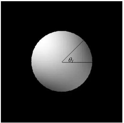
3.1 Single Point Source

The observed objects always have different shapes. The most simple situation is when

(42)

a single point source located at (a,θΙ) on the object plane, whose distribution can be

expressed as the delta function,

) ( ) ( ) ,

( _o _o o _o _I

a a r r

f θ =δ − δ θ −θ

(3.1)

By Eq.(2.2), the radial part of this point source is found to be:

I il o o o il I o o o l e a a r d e a a r r B θ π π θ δ π θ θ θ δ δ π − − − ₌ − − − =

∫

( ) 2 1 ) ( ) ( 2 1 ) ( (3.2)

Applying this result into Eq.(2.14), the coefficientC_l_,_nfor this single point source is

described as

( )

il I n l n l n l e z n l n i C θ λ γ + −

+ − − = 2 , )! | (| ! 1 ) ( (3.3) Where z Ra λ π

γ = . When the value ofC_l_,_nis known, the field on the aperture plane could

be obtained by Eq.(2.13). The first five lowest order modes on the aperture plane may be written as,

Λ µ 4 2 0 8 1 2 1 2 1 ) , ( 2 1       +       −

= γ γ

θ λ R r R r r

zE (3.4a)

( )

₋ µ ₋

( )

₋ µ _±Λ

= ± ± ± ±

± θ γ θ θ γ θ θ

λ i _I i i _I i

e e R r i e e R r i r

zE ₁ 1 1( )3

4 1 ) ( 2 1 ) , ( 2 1 (3.4b) Λ µ µ

µ θ θ _γ θ θ

γ θ

λ 2 2

4 2 2 2 2 12 1 4 1 ) , ( 2

1 i I i _e i _I_e _i

R r e e R r r

zE_± ± _ ±

     +       − = (3.4c)

( )

_γ µ θ θ _µ_Λ

θ

λ 3 3 3

3

3 ( )

12 ) , ( 2

1 i _I i

e e R r i r zE ± ± ± −

= (3.4d)

Λ µ

µ θ θ

γ θ

λ 4 4

4 4 48 1 ) , ( 2

1 i _I i

e e R r r

zE_±  ±

(43)

The total field of the source at the aperture plane is the sum of each mode

∑ ∑

∑

+∞ −∞ = +∞ = +∞ −∞ = = = l n n l l

l r E r

E r

E( , ) ( , ) ( , )

0

, θ

θ θ

(3.5)

Because the dominant modes are lowest modes, here just make a summation of mode

from l=-4 to l=4 as approximation. Thus, the field at the aperture plane of a single

point source is expressed as:

(

)

(

)

(

)

(

)

(

I

)

µΛ

I I I I I l l l p R r R r R r R r R r R r R r R r r E z r zE θ θ γ θ θ γ γ θ θ γ θ θ γ θ θ γ γ θ θ γ θ λ θ λ 4 4 cos 24 1 2 2 cos 6 1 8 1 3 3 sin ) ( 6 1 ) sin( ) ( 2 1 2 2 cos 2 1 2 1 sin ) ( 2 1 2 1 ) , ( 2 1 ) , ( 2 1 4 4 4 3 3 2 2 4 4 −       + −       +       + − − − − −       −       − − + = ≈

∑

= − = (3.6)

This field is superimposed with plane wave and sinusoidal wave with different

[image:43.595.194.401.514.719.2]

frequencies as shown as the following figure.

Fig.3.1 Amplitude of the field at the aperture of a single point source.

(44)

( With πa/λz=0.5 and θI =45 degree)

The first term l=0, n=0 is the most dominant mode, which is a plane wave

component and occupies most power of the total energy as discussed in the Chapter 2.

This component will be diffracted outside the Lyot stop. Note that when a=0, only

plane wave left, other modes equal to zero. That means on-axis point source will be eliminated by Lyot stop completely.

3.2 Binary Points Source

Let's consider the situation when the source is composed with two points separated by

a distance 2a, arranged symmetrically opposed through the optical axis. it can be

described by

)] (

) (

[ ) ( ) ,

( _o _o =δ o− δ θ_o−θ_I +δ θ_o−θ_I −π a

a r y

x f

(3.7)

For the result of the second point source δ(rο−a, θο−θI−π), the calculation is same with Eq.(3.4) except for replacing θI with θI+π, which will cause odd l modes change their signs. Thus, the field of the second point source P' at aperture can be written as

Λ µ

θ γ

γ θ

γ

θ γ

γ θ

λ

4 cos 24

1 2 cos 6

1

8 1 3 sin ) ( 6 1 sin ) ( 2 1

2 cos 2

1 2

1 sin ) ( 2 1 2 1 ) , ( 2 1

4 4

4 3

3

2 2

'

      + 

     +

      + +

+

      −       − −

≈

R r R

r

R r R

r R

r

R r R

r R

r r

zE_p

(45)

The superposition of two points fields at the aperture is expressed as the sum of

modes of each source. Note that odd l modes will be canceled out. For example, if

θI=0, this superposition is expressed as:

Λ + 

     +

      +       + 

     −       − =

∑

) 4 cos( 12

1

) 2 cos( 3

1 4

1 ) 2 cos( 1

) , ( 2

1

4

4 4

2 2

θ γ

γ θ

γ γ

θ λ

R r

R r R

r R

r r

E

z _l

(3.9)

Because the odd terms are vanishing and cos function is an even function, this field

function is even. Fig. 3.2 describes this field pattern when (πa/λz)=0.5. This solution

is in agreement with the expected Fraunhofer diffraction pattern:

( )

n n

n z

y z x o o

r z a n

r z a

y x f FT z

y x zE

2

0 ,

cos 2

! 2

1 cos

2 cos

} ) , ( { 2 1 ) ; , ( 2 1

   

  − =    

  = ≅

∑

∞ =

θ λ

π θ

λ π λ

λ λ

(3.10)

[image:45.595.188.407.508.726.2]

Thus, this result helps refine the previous assumptions is proper.

(46)

As discussed earlier, the OVC with a nonzero even m vortex charge makes the l=0 ,n=0 component in Eq. (3.9) diffracted outside the reimaged pupil radius. The Lyot stop prevents

this plane wave mode from propagating any further through the system. That is, the most

leading component, which makes the two sources unresolvable, can be removed. In this way,

imaging system can spot the observed object more precisely. Now, let's see how to realize it step by step.

By applying the Cl,n value Eq.(3.3) into Eq.(2.20), the field at the Lyot stop from

each point source is not hard to obtain. When the vortex lens in the OVC with vortex charge m=2, the field from the first point source δ(a,0) at the Lyot stop planeG and 2_p

the second point source δ(-a,0) G are separately written as 2_p_'

( )

 �