Nondestructive Evaluation Of Corrosion Damage In Reinforced Concrete Aged Slab Specimen

(1)

University of South Carolina

Scholar Commons

Theses and Dissertations

2018

Goodness of Fit via Residual Plots in Item

Response Theory

Bryonna Bowen

University of South Carolina

Follow this and additional works at:https://scholarcommons.sc.edu/etd Part of theStatistics and Probability Commons

This Open Access Thesis is brought to you by Scholar Commons. It has been accepted for inclusion in Theses and Dissertations by an authorized administrator of Scholar Commons. For more information, please [email protected].

Recommended Citation

Bowen, B.(2018).Goodness of Fit via Residual Plots in Item Response Theory.(Master's thesis). Retrieved from

(2)

Goodness of Fit via Residual Plots in Item Response Theory

by

Bryonna Bowen

Bachelor of Arts

Brigham Young University, 2015

________________________________________________

Submitted in Partial Fulfillment of the Requirements

For the Degree of Master of Science in

Statistics

College of Arts and Sciences

University of South Carolina

2018

Accepted by:

Brian Habing, Director of Thesis

David Hitchcock, Reader

Maureen Petkewich, Reader

(3)

ii

(4)

iii

Acknowledgements

I am very grateful to the many people who helped me complete this thesis.

Foremost, I would like to thank my family for their encouragement and for David

Edwards for always being there for me and his unwavering support.

I would like to express my appreciation and gratitude to my advisor, Dr. Brian

Habing. He always took the time to help me and support me. His flexibility in schedule

allowed me to complete this project. Brian prepared me with the background and

academic knowledge I needed for this project and gave me the programming input

when I needed it the most. He encouraged me to always press forward.

I would also like to thank Dr. David Hitchcock for his long lasting support and

constant willingness to lend a hand when asked. The courses I took from him giving me

a stronger academic background and I’m grateful he was willing to serve as a committee

member. I would also like to thank Maureen Petkewich for her willingness to serve as

(5)

iv

Abstract

Goodness-of-fit criteria developed for the evaluation of item response functions

have been examined by many scholars using different theories and criteria. A number of

potential graphical analysis approaches, such as residual plots, have been described in

literature, but have received little attention from researchers. While many tests of

goodness-of-fit are available, those that incorporate the analysis of residuals may be

most useful. The unmistakable presence of a pattern in the residual plot for the logistic

model item response functions even when we know the model fits raises a red flag up

and calls for greater analysis. This study explores different methods to improve residual

plots for a 3-Parameter logistic model and determine if residual plots are truly useful in

(6)

v

List of Figures

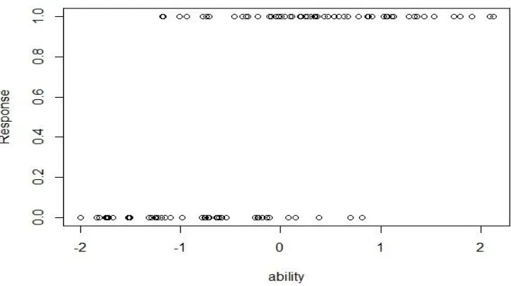
Figure 1.1: Plotting Examinees’ Ability vs. Responses ... 4

Figure 1.2: General Item Response Function Curve ... 4

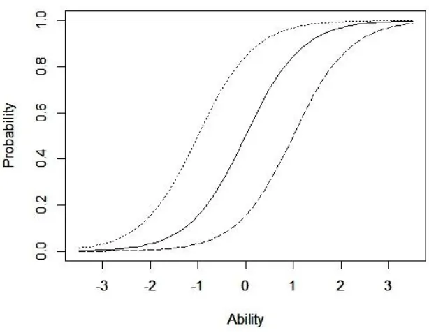
Figure 1.3: Examples of items following the Rasch model ... 10

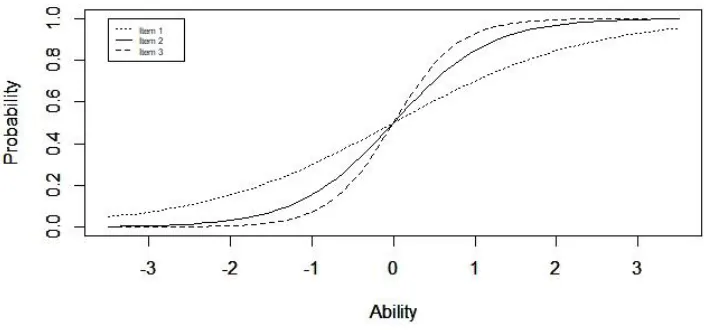
Figure 1.4: Examples of 2PL Items with the Same Difficulty but Varying Discriminations ... 12

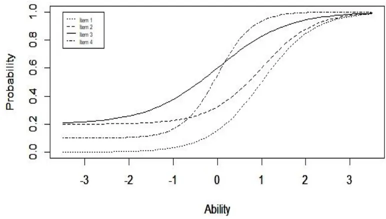
Figure 1.5: Example of 3PL Items with Varying Parameters ... 14

Figure 3.1 Model Predicted Ability vs. Simulated Ability Levels ... 23

Figure 3.2: Ability Divided Evenly by Axis ... 24

Figure 3.3: Thetas Divided Evenly by Examinee Data ... 24

Figure 3.4: Predicted and Observed Probabilities 3PL as 3PL ... 26

Figure 3.5: Standardized Residual Plot 3Pl as 3Pl ... 26

Figure 4.1: Residual Plots for Item 21 Based on Quadrature Interval Type ... 32

Figure 4.2: Item 17 Standardized Residual Plots for Varying Numbers of Quadrature Points ... 33

Figure 4.3: Item 32 Standardized Residual Plots with a Prior and with No Prior ... 35

Figure 4.4: Standardized Residual Plots using Different Quadrature Calculation Methods ... 36

Figure 4.5: Item 7 Standardized Residual Plots using Varying Methods for Quadrature and Observed Calculation ... 37

Figure 4.6: True Model vs. Incorrect Model Standardized Residual Plots for Item 12 .... 38

(8)

vii

Figure A.2 Residual Plots for Item 12 Based on Quadrature Interval Type ... 45

Figure A.3: Residual Plots for Item 17 Based on Quadrature Interval Type ... 46

Figure A.4: Residual Plots for Item 32 Based on Quadrature Interval Type ... 46

Figure A.5: Item 7 Standardized Residual Plots for Varying Numbers of Quadrature Points ... 47

Figure A.9: Item 7 Standardized Residual Plots with a Prior and with No Prior ... 49

(9)

1

Introduction

In order for education levels and academic abilities to be compared across

classrooms, school districts, and state lines, standardized testing has become

increasingly prominent. The most commonly used method to analyze these types of

tests is item response theory (IRT). Consider a standardized math test; ideally, the test

measures a student or examinee’s math ability, or in multidimensional cases the test

can be broken down to measuring various math abilities such as algebra, geometry, and

trigonometry. In either case, analysis models use test responses to simultaneously

estimate item characteristics and examinee abilities.

Various models have been developed to improve the accuracy of estimation and

analysis for measuring tests and creating predictions. However, one of the primary

assumptions for all item response models is that their benefits are only valid if the

model fits properly. Addressing the goodness of model-data fit is therefore, a vital

component to ensuring the appropriate model is selected. The literature available on

model-data fit in IRT is still unsettled as to what constitutes the optimal approach.

Residual plots are used as a standard of measurement for the goodness-of-fit

from a given model. Randomness in the pattern of residuals indicates a good fit, while

(10)

2

U-shape in the residuals for a linear regression points toward a non-linear model as a

better fit. Many residual plots for IRT models show a clear pattern. Does the pattern in

IRT residual plots indicate a poor model-data fit even if all model assumptions are met?

Are there different ways to break up the data and improve the residual plots? If so, what

are the ways? This thesis explores a ways to attempt to improve the residual plots for

IRT parametric models.

The following chapters provide a brief overview of the basics from item response

theory, and the most widely used parametric monotone homogeneity models. Next, an

overview of the IRT goodness-of-fit literature and previous studies will be included. The

current study will then be explained in detail and the results of the study analyzed.

(11)

3

Chapter 1: Item Response Theory

In a world of countless tests measuring achievement, aptitude, and personality,

the analysis of standardized tests is growing rapidly in interest and frequency. Such tests

in education are used to determine if students meet educational standards. For

instance, the ACT, SAT, GRE, MCAT, etc. are all tests used to determine students’

knowledge in targeted areas. While the construction and evaluation of these tests are

subject to various shortcomings, psychometricians use item response theory (IRT) as the

standard set of statistical tools to analyze them.

Item response theory (IRT) is a class of methods of latent variable measurement

models. In a binary test an examinee either gets the question correct or incorrect1.

Plotting observed responses versus ability of the examinee would create essentially

useless graphical representation due to the data’s dichotomous nature (see Figure 1.1).

Mathematical models attempt to describe the relationship between the responses to

the items (i.e. questions) on a test or questionnaire and the underlying latent trait(s)

that the test is designed to measure. Mathematical models known as item response

functions (IRFs) express the probability of an examinee getting an item correct as a

function of the latent ability of the examinee. Similar to logistic regression, the item

1

(12)

4

response function is s-shaped and plots the proportion of correct responses as a

function of the ability in question. An example of an IRF is shown in Figure 1.2.

Figure 1.1: Plotting Examinees’ Ability vs. Responses

(13)

5

The parameter of interest is a latent ability, meaning an ability that is present

but is not apparent, which can also be construed as the existing potential of an

examinee. IRT is based on the premise that (1) an examinee’s performance on a test

item can be predicted by a set of abilities; and (2) the relationship between the

performance of an examinee on an item and the underlying ability can be described by

monotonically increasing item characteristic curve or item response function

(Hambleton and Swaminathan and Rogers, 1991).

IRT models have a long history with many of the central ideas being established

as far back as the 1940s and 1950s (Lawley, 1943; Tucker, 1946; Lazarfeld, 1950; Lord,

1952). Many experts consider the earliest complete application of IRT to be that of

Birnbaum (1968) in a special section of Lord and Novick (1968). Computers and software

caught up with the theory by the 1980s when it became possible to estimate

parameters for problems of meaningful size in reasonable amounts of time. Since then

there has been further research in IRT, including but not limited to creating new models,

forming new methods of estimation, and writing new advanced software.

When a given IRT model fits the test data there are several desirable features

obtained. One distinguishing features of IRT is the property of invariance of item and

ability parameters. The invariance property is even occasionally referred to as the

cornerstone of IRT (Hambleton, Swaminathan, and Rogers, 1991). The property of

invariance implies that the model parameters in IRT do not depend on the ability

distribution of the examinees and that the set of test items is independent from the

(14)

6

Rogers (1985) features of the IRT include: (1) item parameter estimates are independent

of the group of examinees sampled from the population of examinees, (2) examinee

ability estimates are independent of the particular choice of test items used from the

population of items, and (3) a statistic indicating the precision of each examinee’s ability

estimate is known.

Although these features are compelling, as with any mathematical model there

are a set of assumptions about the data which must be met in order to obtain these

qualities. It is also important to note that the extent to which these advantages may be

obtained in practice is determined by how well the test data and the model “fit”.

Assumptions of Item Response Theory

Given that items on a test are dichotomous (2 categories: correct or incorrect)

then a common set of assumptions for an item response theory model is (Swaminathan

& Rogers, 1995):

1. Ability (𝜃) is unidimensional

2. Local Independence

3. Monotonicity

Unidimensionality is the first assumption. The most commonly used IRT models

assume that a test is only measuring a single ability. For example, a constructed math

test attempts to measure examinee’s math ability. However, if there are algebra and

geometry and trigonometry questions then each of these subcategories of math are

additional dimensions. A unidimensional test would measure only one of these abilities

(15)

7

nearly impossible to meet due to the nature of constructing ability. For instance, a word

problem on a math test may measure math ability, but one’s reading comprehension is

also a factor. There are almost always multiple abilities involved; however, the

assumption is that one particular ability dominates the measurement, and is therefore,

considered the measured ability.

The second assumption is local independence. This means that responses are

independent given the ability of an examinee. In other words, one question on the test

does not affect the examinee’s answer on another question of the same test. Each

question is therefore pairwise independent from all other questions on the test. This

can be mathematically written as

𝑃(𝑈₁= 𝑢₁, 𝑈₂ = 𝑢₂, … , 𝑈_𝑛 = 𝑢_𝑛|𝜃) = 𝑃(𝑈1 = 𝑢1|𝜃) ∗ 𝑃(𝑈2= 𝑢2|𝜃) ∗ … ∗ 𝑃(𝑈𝑛 = 𝑢𝑛|𝜃).

The item response function is the probability of response ui occurring for an examinee

with ability (𝜃) to item i. It follows that the examinee’s ability being measured is the

only aspect determining the probability of that examinee getting a particular item

correct. However, Jannarone’s (1986) conjunctive item response models introduce an

alternative model where items are not necessarily locally independent.

Monotonicity is the final assumption. This means that as the examinee’s ability

increases the probability of responding correctly to an item also increases. This seems is

intuitive—if an examinee knows a great deal about algebra he or she is more likely to

get an algebra question correct compared to someone who has little knowledge of

algebra. This assumption of monotonicity is not required in all IRT models, and its

(16)

8

With these three assumptions, a dichotomous item exam following the

monotone homogeneity model stochastically orders ability by the observed total score.

This means that for a fixed ability, 𝜃∗,

𝑃(𝛩 > 𝜃∗|𝑆 = 𝑠₁) ≤ 𝑃((𝛩 > 𝜃∗_{|𝑆 = 𝑠}

2) for all 𝑠1 < 𝑠2.

Stochastic ordering is a property of the minimum model necessary for monotone

homogeneity models and implies that the higher your sum score, the more likely you

are to have a higher ability (𝜃).

Unidimensional Logistic Models

The logistic models included in the research take on some variation of the following

general form

𝑃𝑖(𝜃) = 𝑐𝑖+

1 − 𝑐_𝑖

1 + 𝑒−1.7𝑎𝑖(𝜃−𝑏𝑖), 𝑖 = 1, 2, … , 𝑛

The probability that an examinee with ability θ correctly answers item i is

represented by𝑃𝑖(𝜃). The ability, represented by 𝜃, typically follows a standard normal

distribution (mean equal to 0 and standard deviation of 1).As with all probabilities, the

probability of answering an item correct is given on a range from 0 to 1. The higher

𝑃𝑖(𝜃) is the greater the probability an examinee of ability 𝜃 has of getting item 𝑖 correct.

The discrimination parameter is given by 𝑎𝑖 and is proportional to the slope at

𝜃 = 0 of the item response function. Discrimination of an item refers to how well the

item separates low and high ability examinees. No discrimination (𝑎𝑖= 0) is the

equivalent to flipping a coin, and negative discrimination indicates that the question is

doing the opposite of what you want, such that the higher ability examinees get the

(17)

9

discrimination factors range from 0 to 2 since it is rare that the discrimination factor is

ever greater than 2.

The item difficulty parameter is given by 𝑏_𝑖 and measures how hard or difficult

the item is. The larger 𝑏_𝑖 gets the more ability an examinee needs to get the item

correct (i.e. a harder question). It is the inflection point of item response functions.

The guessing parameter is given by 𝑐_𝑖 and indicates the lower asymptote in the 3

Parameter Logistic (PL) model. The guessing parameter shifts the item response

function to account for guessing. Since the function is based on a multiple choice items,

individuals may not know the correct answer yet still give the correct answer; this

means they may have greater probability of answering the item correct despite a low

ability.

Additionally, we see the notation including the number of items on the test given

by n. And the value of 1.7 in the exponent of the denominator is a standardizing

constant such that it assures that the logistic models and the normal ogive will never

differ by more than 0.01 (see Haley, 1952 as cited by Birnbaum, 1968) .

Rasch Model

The most basic IRT model is the Rasch model (1960) also known as the

one-parameter logistic (1PL) model. It follows the form:

𝑃_𝑖(𝜃) = 1

(18)

10

The Rasch model has a fixed discriminating factor (𝑎_𝑖=1) meaning that all items

modeled will have the same slope. It is therefore assumed that all items distinguish

between all examinees equivalently and that all items are equally related to what ability

the test is measuring. This model is popular for many psychometricians because items

are easier or harder for everyone (i.e. the slopes don’t cross) making the model

straightforward. Figure 1.3 shows three different items each of varying difficulty but as

previously explained, their slopes do not intersect meaning that there is a clear

distinction between which item is more difficult for everyone and which item is easiest

for all examinees (i.e. Hambleton and Swaminathan, 1985).

(19)

11

Another reason the Rasch Model is often used is because if ability is estimated

using maximum likelihood methods, it is not necessary to know whether the examinee

got each item correct or not; a sufficient statistic, 𝑆 = ∑𝑛_𝑖=1𝑈_𝑖, the sum total score is all

the information needed to estimate 𝜃. This model is ideal for explanations to individuals

with little statistical understanding—such as parents and legislators—because all

examinees with the same S will have the same estimated ability, 𝜃̂ (Rasch, 1980).

However, there are limitations to the Rasch model. For example, the Rasch model does

not account for guessing hence 𝑐_𝑖=0. Furthermore, some questions tend to be more

discriminating than others in practice, which is not taken into account with this model.

In essence, its simplicity is also its weakness.

Two Parameter Logistic Model

Birnbaum’s (1968) two parameter logistic (2PL) model follows the following

general form:

𝑃_𝑖(𝜃) = 1

1 + 𝑒−1.7𝑎𝑖(𝜃−𝑏𝑖), 𝑖 = 1, 2, … , 𝑛

This 2PL function is similar to the Rasch model but adds a parameter accounting

for the discrimination factor of each item. The discrimination parameter, ai, is

proportional to the slope in the IRF. An item with larger ai value has a steeper slope

which indicates higher discrimination factor; therefore, such an item will do better at

separating higher ability examinees from lower ability examinees. With items allowed to

have varying discrimination values, the item response functions of different items may

(20)

12

Figure 1.4: Examples of 2PL Items with the Same Difficulty but Varying Discriminations

By examining Figure 1.4 we see all three items have the same difficulty, bi =0.

Item 2 has the same discrimination factor, or slope, as the Rasch model (𝑎₂ = 1). Item 1

has a lower item discrimination (𝑎₁ = 0.5) and item 3 has a high discrimination factor

(𝑎₃ = 1.5). To interpret this, we can say that item 1 is easiest and item 3 is most difficult

for examinees with low ability. However, for examinees with high ability we see that

item 3 is easiest and item 1 is most difficult at these higher abilities. Therefore, it cannot

be said that one item is strictly easier or more difficult than other items. While this

distinction complicates analysis, it also provides more information about the items by

including the discrimination factor. Estimation in the 2PL model is harder because there

is not a sufficient statistic for 𝜃. Neither the Rasch model nor the 2PL model account for

examinees guessing on items. To include a guessing factor we must introduce the 3PL

(21)

13

Three Parameter Logistic Function

The more complicated but still commonly used IRF is the 3 parameter logistic

(3PL) model (Birnbaum, 1968). The 3PL model accounts for the possibility of examinees

guessing on items. The generalized form of the 3PL model follows:

𝑃_𝑖(𝜃) = 𝑐_𝑖+ 1 − 𝑐𝑖

1 + 𝑒−1.7𝑎𝑖(𝜃−𝑏𝑖), 𝑖 = 1, 2, … , 𝑛

In both the Rasch and the 2PL models, the guessing parameter 𝑐_𝑖 = 0; in the 3PL

model the range of 𝑐_𝑖 is theoretically from 0 to 1, but is frequently thought of as being

0.2(which would correspond to a multiple choice question with five response

categories). The guessing parameter manifests itself via a lower asymptote in the IRF.

This means that an examinee with hypothetically no ability still has a probability equal

to 𝑐𝑖 of getting the item correct. This is relevant because many tests used for IRT are

multiple choice and even if an examinee chooses a random answer there is still some

chance that he or she guesses correctly. In Figure 1.5 we see an example of four

different 3PL items.

The addition of a guessing parameter is very evident in the graph of Figure 1.5.

The lower asymptote is for item 1 is 0, like the 2PL model, but item 4 (𝑐𝑖 = 0.1) and

items 2, 3 (𝑐𝑖 = 0.2) include guessing parameters. Note that item 4 has a lower

guessing parameter than item 2 and item 3, which means that examinees with lower

abilities have a lower chance of answering item 4 correctly than they do item 2 or 3 but

(22)

14

the items above and therefore, the same inability to determine an overall easier or

harder item from the 2 PL model is also in effect here

(23)

15

Chapter 2: Residual Plots and Literature Review

Residual Plots

Given that we now have a few monotone homogeneity models to choose from

the following questions come to mind: How can you determine if a model fits the data?

If there are multiple potential models to use, how can you tell which one of the models

is most appropriate? What do we do when we have our data and we think a certain

model fits? As with most analytical methods, we want some statistical way to go

through and determine what model we should use for the data.

Direct diagnostic plots for the response variable are rarely useful because

observations and response variables may be on different scales based on the levels of

the predictor variable. Instead, the residuals are examined to determine the diagnostics

for the dependent variable (Kutner et al., 2005). Residuals are the calculated differences

between the predicted and observed values, typically for each individual or unit. The

observed error, regarded as the residual, is defined as

𝑒_𝑖 = 𝑌_𝑖− 𝑌̂_𝑖

Residuals are often presented as standardized or studentized residuals, meaning

that the residual is normalized by the estimate of its standard deviation at each

predicted value. This allows us to compare residuals at different data points when they

are calculated to be on the same scale. The following form of standardization is

(24)

16 𝑒_𝑖∗= 𝑒𝑖 − 𝑒̅

√𝑀𝑆𝐸

where √𝑀𝑆𝐸 is an estimate of the standard deviation of the residual. Hence, the

statistic ei is referred to as the studentized or semistudentized residual (Kutner et al.,

2005). The unknown true error, εi, is given as:

𝜀_𝑖 = 𝑌_𝑖 − 𝐸{𝑌_𝑖}

In standard linear regression, the error terms, 𝜀𝑖, are assumed to be independent

normal random variables, with mean 0 and constant variance𝜎2. These properties

assumed for 𝜀𝑖 should be reflected by the observed residual (or studentized residual) if

the model is appropriate (Kutner et al., 2005).

A residual plot is a graph showing the residuals on the vertical axis and the

independent variable values on the horizontal axis. If the residual plot shows no pattern,

or in other words the residuals appear to be random, then we typically assume that the

model is appropriate for the data. Otherwise, we usually believe another model is more

appropriate, often times a non-linear or in the case of IRT perhaps a nonparametric

model.

In general, the ideal residual plot has (1) residuals that are fairly symmetrically

distributed and with mean equal to 0 and (2) no clear patterns in the plot. However, as

George Box famously stated, “essentially, all models are wrong, but some are useful”

(1976). So while the model may not be perfect and the residuals look like the model can

improve, a decent model is better than no model at all. In practice “how good is good

enough?” is a judgment call everyone has to make depending on the intent of the

(25)

17

surprising that item response model researchers have not given residuals more

attention.

Previous Research

Testing the goodness-of-fit of IRT models is essential to validating IRT models.

Goodness-of-fit methods have lagged behind estimation methods for IRT models for

some time (van der Linden & Hambleton, 1997; Maydeu-Olivares, 2013). At first overall

goodness-of-fit tests involved contingency tables and frequencies (Bishop, Fienberg, &

Holland, 1975). Over time several goodness-of-fit tests developed, including the more

notable Pearson’s chi-squared (𝜒2) test and Likelihood ratio test (𝐺2). Many scholars

have described the use of these statistics with IRT models and done in-depth research

for which model assumptions appear to be violated and how the model assumptions

affect the goodness-of-fit statistics (Lord & Novick, 1968; Thissen, 2013;

Maydeu-Olivares, 2013). However, there are several other methods and statistics used to assess

goodness-of-fit in IRT.

One of the primary concerns of goodness-of-fit for IRT parametric models is that

item bias affects the parameter of interest, i.e. ability. In such cases there is an “effect of

misspecification on the goals of IRT analysis,” undermining the features previously

mentioned in Chapter 1 (Obereki and Vermut, 2013). Therefore, understanding the

efficiency of of-fit tests or having the ability to accurately interpret

goodness-of-fit statistics is of paramount importance. A common approach to assessing IRT

models’ goodness-of-fit is analyzed in the research by using comparing methods of

(26)

18

scholars, propose using posterior probabilities for responses across ability levels rather

than using the traditional method of cross-classification of examinees and point

estimates of θ (Stone, Mislevy, & Mazzeo, 1994; Donoghue and Hombo, 1999, 2001).

Stone, Mislevy, and Mazzeo argue that the goodness-of-fit statistics approximated

under the null distribution deviate according to the uncertainty in ability estimation.

Donoghue and Hombo derived a distribution of the fit statistic in order to perform

hypothesis testing. However, Hambleton and Swaminathan (1985) discuss other

validation techniques and dispute that too much reliance has been placed on model fit

statistical tests resulting in erroneous decision and serious flaws. This weakness in

statistical tests of model fit has since become well-known and analyzed more deeply.

A comparison of observed and expected frequencies across score levels with a

fit statistic that does not use ability estimates has been provided by Orlando and Thissen

(2000). Sources of misfit have also been assessed using modification indices such as

Lagrange multiplier tests, where statistics for residual means and covariances are tested

(Maydeu-Olivares, 2013). However, many problems with types of goodness of fit tests

have been thoroughly discussed in existing literature (see Hambleton & Swaminathan,

1985; Mislevy & Bock, 1990; Muraki, 1997). In particular, these scholars present

concerns about the inefficiencies and the issues with chi-square tests in general

(Hambleton & Swaminathan, 1985; Bock, 1989) and the number of subgroups

representing the “threat” (Muraki, 1997).

A number of potential graphical analysis approaches have been described in

(27)

19

goodness-of-fit are available as evident from the extensive research done; however,

those that incorporate the analysis of residuals seem most useful (Hambleton &

Swaminathan, 1985; McDonald, 1982). Wright and Stone (1979) compute a

goodness-of-fit statistic based on the residuals, but illustrate the difficulty of seeing how the

magnitude of residuals could be directly correlated on the fit of the model. The shape of

item characteristic curves and estimated abilities from different models compared to

the raw scores is a visual method of seeing approximate model-data fit (Lord, 1970). It

was further determined by Lord (1974) that this relationship—model estimates versus

raw data—may not be perfect but should be highly correlated.

Hambleton and Swaminathan (1985; Hambleton, Swaminathan, & Rogers, 1991)

have presented examples of residual plots used in assessing goodness-of-fit. They state

that the “observed pattern of standardized residuals shown is due to the fact that the

item is less discriminating than the average level of discrimination adopted for all items

in the model” (Hambleton, Swaminathan, and Rogers ,1991). While clear improvements

are gained by using the two-parameter and the three-parameter models, the pattern in

the standardized residual plot is less evident but still clearly exists. The unmistakable

presence of a pattern in the residual plot for the IRF even when we know the model fits

raises a red flag up and is the call for this study.

While Hambleton, Swaminathan, and Rogers present a number of alternative

residual analyses—including: observed and expected proportion correct for items,

standardized residual plots, frequency distributions of standardized residuals , and

(28)

20

research uses only the first two methods (observed and expected proportion correct for

items, standardized residual plots) and focuses on, if possible, how the standardized

residual plots can be improved to help determine goodness of fit of item response

(29)

21

Chapter 3: Current Study

While researchers have evaluated traditional IRT goodness-of-fit tests via test

statistics and methods, this research explores possible improvement to residual plots

that assess IRT models goodness-of-fit. In designing a goodness-of-fit investigation for

IRT models, Stone and Zhang’s (2003) five step outline is used. Their outline of the

traditional approach to assessing IRT model fit includes:

1. Estimate the item and ability (𝜃) parameters

2. Form a small number of ability subgroups

3. Construct an observed score response distribution for each ability subgroup

4. Form an expected score response distribution for an item using the IRT

model across score categories

5. Compare predictions and observed score responses

Here we will also include a sixth step from Hambleton and Swaminathan (1985) to

address the fit between different models.

6. Determine the appropriateness of the intended application

Before we can proceed with the outline approach it is necessary to obtain or

create data to analyze. Researchers have used simulation studies as a valuable method

to learn about item response models and how different applications of IRT compare

(30)

22

Swaminathan, 1985). According to Hambleton and Swaminathan (1985) it is possible to

simulate data with known properties to determine how well various models recover the

true parameters. In this case simulated data is generated to fit a 3PL model in R;

therefore, we have data with a known model that should fit and the model assumptions

can be assumed to have been met since this is a simulation study with a known model

fit. The true plot or true model in this study is a three-parameter logistic model.

The simulation used includes a test with 32 items and 2000 examinees. The

discrimination parameters (ai) were set with a range of (.75, 1.5) in intervals of .05. The

difficulty parameters (bi) were was set from (-1,1) in intervals of 0.25. The guessing

parameters were all set equal to 0.2, which is a very typical guessing parameter value in

simulation studies. This simulation is not based off a specific test, or other results but

rather attempts to cover general IRT data to explore the residual plots.

To follow the outline above we had to first, estimate the item and ability (𝜃)

parameters. PARSCALE (du Toit, 2003) statistical analysis software was used to fit a 3PL

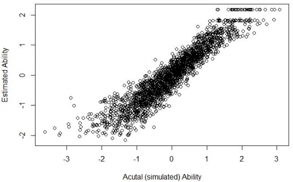
model to the simulated data. In practice, the simulations created should reflect the

actual test parameters. This can be verified by Figure 3.1 which compares the actual

ability values we simulated to what our model’s ability estimates are, and appears to be

(31)

23

Figure 3.1 Model Predicted Ability vs. Simulated Ability Levels

Secondly, a small number of ability subgroups is formed. Ability subgroups are

represented by quadrature points and are calculated here using two different methods.

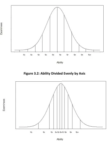
Subgroups can be calculated by evenly dividing the range of ability into equal intervals

(see Figure 3.2) or they can be calculated by putting an equal number of examinees

with similar abilities into each interval (see Figure 3.3). Quadrature points using the

midpoint rule are used such that quadrature point i is calculated by:

𝑞_𝑖 =𝑎𝑖 + 𝑏𝑖 2

where 𝑎𝑖 is the lower bound of the interval and 𝑏𝑖 is the upper bound of the

interval. In actuality, we would not have a bunch of people with tied thetas (abilities),

but for the purpose of simplicity we use quadrature points to represent approximate

(32)

24

Figure 3.2: Ability Divided Evenly by Axis

Figure 3.3: Thetas Divided Evenly by Examinee Data

Third, an observed score response distribution for each ability subgroup is

constructed. The responses of examinees are binary (0 or 1) yet the predictor

(probability of answering item correctly) is continuous. Therefore, in order to make the

plot work the predictor can be calculated as the percentage of examinees in a set range

(33)

25 𝑃[𝑈𝑗𝑖 = 1] = 𝑃̂𝑗𝑖 = 𝑐̂𝑖+

1 − 𝑐̂_𝑖 1 + 𝑒−1.7𝑎̂𝑖(𝜃̂𝑗−𝑏̂𝑖)

where,

𝑃̂_𝑗𝑖 is the percentage of people in subgroup j who get item i correct,

𝑎̂_𝑖 is the predicted discrimination parameter for item i,

𝑏̂𝑖 is the predicted difficulty parameter for item i,

𝑐̂𝑖 is the predicted guessing parameter c for item i, and

𝜃̂_𝑗 is the predicted ability for the quadrature point j

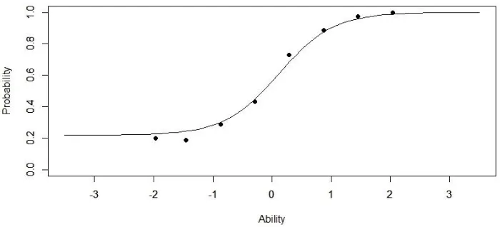
This percentage from the data should be close to the model curve or IRF for the correct

model (See Figure 3.4).

Fourth, expected score response distribution for an item using the IRT model are

formed across score categories. Since our data is simulated to follow a 3PL we know

that the parameters estimated from Parscale should closely represent a 3PL model (See

Figure 3.4).

Fifth, the predictions and observed score responses are compared. To do this we

plot the IRF from the data and the IRF for the estimation for an item. Looking at Figure

3.4 we see that the estimated values follow the true model well. However, in statistical

analyses we rarely look at just “x vs. y plots” due to scaling. Instead, we evaluate

goodness-of-fit via residual plots (See Figure 3.5). The residuals can be found in Figure

3.4 if one were to draw a line of the shortest distance between the observed points and

(34)

26

scaling and for ease of viewing the residuals we plot residuals on a graph where the

horizontal axis is the ability and vertical axis is the residual value.

Figure 3.4: Predicted and Observed Probabilities 3PL as 3PL

(35)

27

There is a clear pattern seen in the residual plot in Figure 3.5. The low ability

values have negative standardized residuals. And as ability increases the standardized

residuals are increasing, ending with high positive residuals for the high ability values.

This pattern is discouraging because it indicates a poor model fit, even though the

model used is the “true” model (3PL model for 3PL data). This means that there is either

a mistake in the calculations for the residual plot or we need to interpret it differently

than what we usually think. There are many options behind these plots which may be

investigated and are addressed in this study.

First, how do we determine the manner in which to define and create

quadrature points? At the ends of the ability scale in Figure 3.4 the curve is fairly flat,

indicating that changing groups of examinees in this area may not change the estimates

significantly. In the middle of the curve, the slope is steep; suggesting that the range of

thetas or examinees in a subgroup will cause variation on the estimates (probability of

getting item correct). One way to divide thetas up is divide the line up into equal

intervals on the axis. We can also divide the theta up by the number of examinees in an

interval. Classifying examinees with similar estimated abilities (𝜃̂) together with either

method seems reasonable.

Second, how many subgroups should be created for abilities? One thing to

consider is that while using many subgroups increases the accuracy of the model

estimates for a given value of ability, smaller subgroup populations also cause large

(36)

28

Third, the method of modeling may be off. When Bayesian estimation is used,

examinee estimates are pulled toward the middle. The prior probability distribution

pulls the estimated abilities in to the mean of the prior (typically a standard normal

distribution with mean=0, sd=1). If the estimated abilities are being pulled in

considerably from the true values then the estimated abilities are less compatible with

the observed. A greater difference between the estimated and the observed values

means the residuals will be larger. Thus, having a prior could affect the residuals.

Finally, a new method of distributing the examinees to the quadrature points will

be explored. By estimating the probability each examinee has of being in any given

quadrature point, we can more accurately represent the data or examinees by

quadrature points. This new method will be explored to determine if calculating

quadrature points differently will improve the goodness-of-fit as shown in the residual

plots.

There are many new things to consider about residual plots for item response

functions that are already well explored or defined for linear regression. Since this thesis

works entirely with simulated data, the “true” model is known and the residual plots

analyzed. However, the only way residual plots are useful is if one knows what they

should look like when the assumptions and model are true. Even if the true model has

satisfactory residual plots, if an incorrect model has similar appearing residual plots then

the residual plots are not helpful in differentiating a model of good fit. This is of

paramount importance because the true model is never known when using real data in

(37)

29

an incorrect model—a Rasch model—will be fit to the simulated 3PL data to determine

(38)

30

Chapter 4: Results

Every item of an exam uniquely contributes to the estimation of an examinee’s

ability. The two main differences for each item are quantified by the difficulty and

discrimination parameters of the items. The difficulty and discrimination of an item may

also strongly influence the residuals. Therefore, at each of the stages of analysis five

different items will be used. The items selected were based on combinations of low and

high discrimination and low and high difficulty parameters. Additionally, three

simulations each based on the same true parameters will be used for each item.

Simulations imitate the randomness and interdependence of real-life data without

having sampling and human error. This idealizes the type of data received and used in

IRT analyses. The use of multiple simulations is to verify that the patterns seen in the

residual plots are not just random by chance, if they occur for a given item for all three

simulations. In each of the following residual plots all three of the simulations are

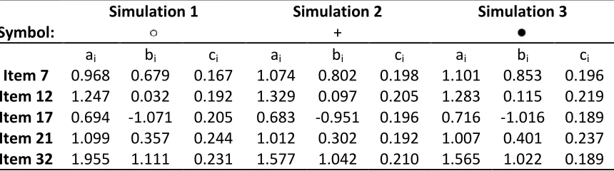
plotted on the same figure. Table 4.1 shows the parameter values of the items for each

simulation used in this analysis and the symbol used for that simulation on each of the

graphs. For each exploration in this thesis, the residual plot for one item is presented in

(39)

31

Table 4.1: Parameter Values for Items Chosen

Symbol:

Simulation 1 Simulation 2

+

Simulation 3

ai bi ci ai bi ci ai bi ci

Item 7 0.968 0.679 0.167 1.074 0.802 0.198 1.101 0.853 0.196

Item 12 1.247 0.032 0.192 1.329 0.097 0.205 1.283 0.115 0.219

Item 17 0.694 -1.071 0.205 0.683 -0.951 0.196 0.716 -1.016 0.189

Item 21 1.099 0.357 0.244 1.012 0.302 0.192 1.007 0.401 0.237

Item 32 1.955 1.111 0.231 1.577 1.042 0.210 1.565 1.022 0.189

Dividing the Thetas (Quadrature Type)

There was not a clear indication of which method of dividing the thetas worked

best. For some items the quadrature points based on the data seemed to have more

randomized residuals plots, which other items indicated using the axis to divide the

thetas was better. If we divide the thetas based on the axis, the intervals are equal in

length, but there will be more examinees included in the middle intervals and in a small

sample there is a chance that the intervals in the tail ends will not have examinees. In

this simulation, the tail ends did not have examinees, meaning that by dividing on the

axis there were 2 fewer quadrature points included on the plots. On the other hand the

thetas could be divided up by the data having an equal number of examinees in each

group. However, dividing theta based on the number of examinees means that some

intervals may be rather large and should not be grouping such differing abilities

together.

There may again be greater issues at the tail ends. Dividing by the data will either

(40)

32

point, and some examinees with lower abilities will be represented by a higher ability

quadrature point; or (2) pull all the quadrature points to the middle of the theta

distribution since that is where the majority of the examinees are. Overall, either

method seems reasonable since they are grouping examinees with similar thetas

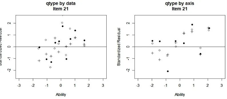
together, but in detail each method has limitations as well. In Figure 4.1 the residual

plots for item 12 are shown where quadrature points are based on division of the axis

and data respectively.

Figure 4.1: Residual Plots for Item 21 Based on Quadrature Interval Type

After examining both residual plots there is a still a clear pattern in either, where

the residuals are negative at the low ability and get progressively higher and more

positive as ability increases. Unfortunately, without a clear indication of which method

is better, we will move forward using the division of examinees into quadrature points

based on the axis since there appears to be slightly less of a pattern in the axis based

(41)

33

Number of Quadrature Points

Continuing to calculate the quadrature points based on the axis, we next looked

at how many quadrature points should be included. While more quadrature points

would indicate a closer fit and smaller residuals, too many groups results in very few

individuals in each group causing the standard deviation to explode. Therefore, with

2000 examinees it seems reasonable to analyze a range of 5 to 30 quadrature points.

Figure 4.2: Item 17 Standardized Residual Plots for Varying Number of Quadrature Points

Figure 4.2 shows the residual plots with varying numbers of quadrature points

for Item 17. When more quadrature points are included the residuals appear more

randomized; however, too many groups also show larger residuals and in theory may

cause inflation of the standard deviation. Therefore, we want as few quadrature points

(42)

34

no two examinees have the same thetas; it seems extreme to analyze dozens of

examinees as if they had the same theta which occurs when only five or ten quadrature

points are used. We conclude that 20 quadrature points appears to be the best number

of quadrature points to include, addressing enough but not too many quadrature points.

With 2000 examinees in this simulation, having 20 quadrature points seems reasonable,

although the number of quadrature points may need to be readdressed with smaller

sample sizes, and calls for additional study.

Effect of Priors

Our next analysis looked at how much a having a prior on the parameters affects

the residuals. Using the same simulated data I used PARSCALE once again to calculate

the estimates without using priors on any of the parameters. Unfortunately, this hardly

changed anything in the data because the simulated data was already similar to what

the standard normal priors would have pulled them towards. It is likely with real life

data and skewed distributions that the prior will have a greater effect on the residuals

than it does in this simulation. Figure 4.3 shows how little change occurred in the

residual plots for item 32.

While the residual plot looks okay on its own in Figure 4.3 there is not a clear

distinction in the residual plots as to whether including a prior improves the model fit

via the residual plots. None of the above typical methods gave clear indication of how to

(43)

35

Figure 4.3: Item 32 Standardized Residual Plots with a Prior and with No Prior Quadrature Calculations

The final exploration introduces two new methods of calculating the quadrature

points. The first method involves calculating an examinee’s probability of being at any

given quadrature point. This calculation may be done because we have the predicted

abilities and their predicted standard errors (se). We can then find the estimated

probability that each examinee is at each quadrature point in a manner similar to part of

the E step in the expectation-maximization (EM) algorithm/Bayes modal estimation of

the item parameters.

In this calculated matrix of probabilities each row represents an examinee and

the sum of each row is equal to 1. Each column represented a quadrature point and

each column adds to the effective number of examinees at that quadrature point. The

data matrix (0=incorrect and 1= correct) is multiplied by the above calculated

quadrature weight matrix resulting in a matrix of the observed total amount of correct

responses at each quadrature point. This matrix must then be standardized in order to

(44)

36

expected total amount of correct responses at each quadrature point. The standardized

residuals are calculated as usual (observed-expected) and plotted. Figure 4.4 shows the

respective standardized residual plot and the original method standardized residual plot

for item 17.

Figure 4.4: Standardized Residual Plots using Different Quadrature Calculation Methods

As evident from the Figure 4.4 the new calculations for the quadrature points

decreases the magnitude of the residuals, but a pattern of negative residuals for low

ability and positive residuals for high abilities can still be somewhat seen, although it is

less of a pattern.

The second method of calculation uses the same above method for calculating

each examinees probabilities for each quadrature point; however, the average theta (𝜃̅)

(45)

37

probability of getting the item correct. This calculation is based on the estimation

procedures of long tests from Mathilda du Toit (2003).

±2√𝑃_𝑖(𝜃̅_ℎ)[1 − 𝑃_𝑖(𝜃̅ℎ)]/𝑁ℎ

where

𝑃𝑖(𝜃̅ℎ) is the probability of correctly answering item i, for the average thetas at

quadrature point h and

Nh is the total number of examinees at quadrature point h.

Figure 4.5: Item 7 Standardized Residual Plots using Varying Methods for Quadrature and Observed Calculation

Figure 4.5 compares the three calculations of residual plots. The original method

is using standard quadrature calculations, the method 1 uses the calculation of the

probability of a given examinee at each quadrature point, and the method 2 uses the

average ability within the quadrature point. Unfortunately, this new calculation of

residuals by using the average ability of each quadrature makes the residuals about the

(46)

38

True model vs. Wrong Model

The only way residual plots are useful is if you know what they should look like

when the assumptions are true. After creating improved residual plots for the

simulations in this study, does it actually help determine the goodness-of-fit for the

model? If the residual plot for the wrong model looks the same as the residuals for the

true model then the goodness-of-fit interpreted from the residual plots in inconclusive.

The true model for real life data is never known; therefore, if the residual plots for a

true model and an incorrect model appear very similar in a simulation, it is unreliable to

assess goodness-of-fit via the residual plots. Using the method of calculating an

examinee’s probability of being at any given quadrature point the true model is

compared to an incorrect model. A wrong model example was estimated using the same

simulated data but instead an incorrect model, a Rasch (1PL) model was fit to the 3PL

simulated data.

Figure 4.6: True Model vs. Incorrect Model Standardized Residual Plots for Item 12

In Figure 4.6 we compare the standardized residual plot of the true model fit

(47)

39

There is a clear indication that the residuals of the true model are closer to zero and the

Rasch model on 3PL data has larger residuals. While there is not a clearly distinctive

pattern differentiation between the two, the magnitude of the residuals can distinguish

between the true model and the incorrect model. If the true model were not known, as

would be the case in real data situation, it may be extremely difficult to determine if a

(48)

40

Conclusion

The ad hoc manipulations to the residual plots may have slightly improved, or

eliminated what was originally determined as worrisome pattern in the residuals.

However, there is not enough distinction between true model and incorrect model to

make goodness-of-fit analysis via residual plots clear without a true model to compare

the incorrect model residuals to. However, as seen in Figure 4.6, the magnitude of the

residuals may be able to be used to determine a model’s goodness-of-fit.

In real life, no data set actually comes from a model, but will be more

complicated in actuality. In order to compare residual plots with real data perhaps the

best thing to do is (1) fit the model in question to the data, (2) simulate data sets based

on the parameter estimates from the real data, (3) create plots of what it would look

like if the model was true from the simulated data, (4) compare the one from real data

to the simulated data. If the real model looks like the simulated model then perhaps

your model fits well. The magnitude of the residuals from a true model to the sample

data can also be compared to help judge goodness-of-fit.

Call for Further Study

Advantages from Item response models are “only obtained in practice… when

there is a close match between the model selected for use and the test data”

(49)

41

determine goodness-of-fit using residuals. To determine if the conclusions of residual

magnitude hold for more general cases, a continuing analysis should be done with a

small sample size simulation, a short exam, and a longer exam. The 2PL model should

also be included to compare to the 3PL and the Rasch models. This study could also be

extended by examining the magnitude of residuals for true vs. incorrect models. The

true model appears to have residuals closer to zero whereas the incorrect model has

larger residuals. Can this be an indication of whether the chosen model fits? Without a

rule of thumb for the how large “good fitting” residuals may be, there is no indication

(50)

42

References

Birnbaum, A. 1968. Some latent trait models and their use in inferring an examinee’s ability. In F. M. Lord & M. R. Novick, Statistical theories of mental test scores. Reading MA: Addison-Wesley.

Bishop, Yvonne M. M., Stephen E. Fienberg, and Paul W. Holland. 1975. Discrete

Multivariate Analysis: Theory and Practice. Cambridge, Massachusetts: The MIT

Press.

Bock, R. Darrell. 1989. A Brief History of Item Theory Response. Educational

Measurement: Issues and Practice 16, no. 4 (winter):21-32.

Box, George E.P. 1976. Science and Statistics Journal of the American Statistical

Association 71: 791-799.

Bustamante, Carlos and Juan Chacon. 2016. Estimation and Goodness-of-Fit in Latent

Trail Models: A Comparison among Theoretical Approaches. Statistical

methodology, no. 33 (December): 83-95.

Dempster, A.P., N.M Laird, and D.B. Rubin . 1977. Maximum Likelihood from Incomplete Data via the EM Algorithm. Journal of Royal Statistical Society. Series

B(Methodological 39, no. 1 : 1-38.

Donoghue, J. R., & Hombo, C. M. 1999. Some asymptotic results on the distribution of an

IRT measure of item fit. Paper presented at the Psychometric Society, Lawrence,

KS.

Donoghue, J. R., & Hombo, C. M. (2001b, April). The effect of item parameter estimation on the distribution of an IRT item‐fit measure. Paper presented at the Annual Meeting of the NCME, Seattle, WA

Du Toit, Mathilda, ed. 2003. IRT from SSI: BILOG-MG , MULTILOG, PARSCALE,

TESTFACT. United States of America: Scientific Software International Inc.

Edwards, Michael C., Li Cai, and Carrie R. Houts. 2018. A Diagnostic Procedure to Detect Departure from local independence in Item response theory models.

Psychological Methods 23, no. 1 (March): 138-149.

Essen, Cyrinus B., Idaka E. Idaka, and Michael A. Metibemu. 2017. Item level diagnostics and model-data fit in item response theory (IRT) using BILOG – MG V3.0 and

IRTPRO V3.0 Programmes. Global Journal of Educational Research 16, no. 2:

87-94.

Hambleton, Ronald K. 1969. An empirical Investigation of the Rasch Test Theory Model.

Unpublished doctoral dissertation University of Toronto.

(51)

43

Hambleton, Ronald K., & Cook, L. L. 1983. Robustness of item response models and effects of test length and sample size on the precision of ability estimates. In D. J. Weiss (Ed.), New horizons in testing: Latent trait test theory and computerized

adaptive testing (pp. 31– 49). New York, NY: Academic Press.

Hambleton, Ronald K., Hariharan Swaminathan, and H. Jane Rogers. 1991.

Fundamentals of Item Response Theory. United States of America:Sage

Publications Inc.

Hambleton, Ronald K., and Hariharan Swaminathan. 1985. Item Response Theory:

Principles and applications. Hingham, MA: Distributor for North America, Kluwer

Boston Boston.

Jannarone, Robert J. 1985. Conjunctive item response theory kernels. Psychometrika 51, no. 3 (September): 357-373.

Kutner, Michael H., Christopher J. Nachtseim, John Neter, and William Li. 2005. Applied

Linear Statistical Models. 5th ed. New York, NY: McGraw-Hill companies Inc.

Lawley, D.N. 1943. The Application of the Maximum Likelihood Method to Factor Analysis. British Journal of Psychology 33, no. 3(January):172-175.

Lazarsfeld, P. F. 1950. The logical and mathematical foundation of latent structure analysis. In S. A. Stouffer, L. Guttman, E. A. Suchman, P. F. Lazarsfeld, S. A. Star, & J. A. Clausen, Measurement and prediction. Princeton: Princeton University Press.

Lord, F. M. 1970. Estimating item characteristic curves without knowledge of their mathematical form. Psychometrika, 35: 42-50.

Lord, F. M. 1974. Estimation of latent ability and item parameters when there are omitted responses. Psychometrika, 39:247-264.

Lord, F.M. 1952. A theory of test Score. Psychometric Monograph, no.7.

Lord, F.M. and Novick. 1968. An analysis of the Verbal Scholastic Aptitude Test using

Birnbaum’s three-parameter logistic model. Educational and Psychological

Measurement, 28: 989-1020.

Lord, F. M., & Novick, M. R. 1968. Statistical theories of mental test scores. Reading MA: Addison-Wesley.

Maydeu-Olivares, Alberto. 2013. Why Should We Assess the Goodness-of-Fit of IRT Models? Measurement 11, no. 3: 127-137.

McDonald, Roderick P. 1982. Linear Versus Nonlinear Models in Item Response Theory.

Applied Psychological Measurement 6, no. 4: 379-396.

Mislevy, R., and Bock, R. D. 1990. PC BILOG 3: Item analysis and test scoring with binary

logistic models (2nd. Ed.). Chicago: Scientific Software, Inc

Muraki, Eiji. 1997. A generalized partial credit model. In W. J. van der Linden & R. K.

Hambleton (Eds.), Handbook of modern item response theory (pp. 153–

164). New York: Springer

(52)

44

Orlando, Maria, and David Thissen. 2000. Likelihood-Based Item-Fit Indices for

dichotomous Item Response Theory Models. Applied Psychological

Measurement 24, no. 1(March): 50-64.

Rasch, G. 1960. Probabilistic Models for Some Intelligence and Attainment Tests. Copenhagen: Danmarks Paedagogiske Institut.

Ree, M.J. 1979. Estimating Item Characteristic Curves. Applied Psychological

Measurement, no. 3:371-385.

Roberts, James S., and James E. Laughlin. 1996. A Unidimensional Item Response Model

for Unfolding Responses from a Graded Disagree-Agree Response Scale. Applied

Psychological Measurement.

Stone, Clement A. and Bo Zhang. 2003. Assessing Goodness of Fit of Item Response

Theory Models: A Comparison of Traditional and Alternative Procedures. Journal

of Educational Measurement 40, no. 4 (winter): 331-352.

Stone Clement A., RJ Mislevy, and J. Mazzeo. 1994. Classification error and goodness-of-fit in IRT models. Paper presented at the annual meeting of the American

Educational Research Association, New Orleans, LA.

Thissen, David. 2013. The Meaning of Goodness-of Fit Tests: Commentary on

“Goodness-of-Fit Assessment of Item Response Theory Models”. Measurement

11, no. 3: 123-126.

Tucker, Ledyard R. 1946. Maximum validity of a test with equivalent items.

Psychometrika 11, no. 1 (March): 1-13.

Van der Linden, Wim J., and Ronald K. Hambleton (Eds.) 1997. Handbook of Modern

Item Response Theory. Springer New York, NY.

(53)

45

Appendix A: Additional Items’ Residual Plots

Quadrature Type: Data vs. Axis

Figure A.1: Residual Plots for Item 7 Based on Quadrature Interval Type

(54)

46

Figure A.3: Residual Plots for Item 17 Based on Quadrature Interval Type

(55)

47

Number of Quadrature Points

Figure A.5: Item 7 Standardized Residual Plots for Varying Number of Quadrature Points

(56)

48

Figure A.7: Item 21 Standardized Residual Plots for Varying Number of Quadrature Points

(57)

49 Prior Effect on Residual Plots

Figure A.9: Item 7 Standardized Residual Plots with a Prior and with No Prior

(58)

50

Figure A.11: Item 17 Standardized Residual Plots with a Prior and with No Prior

(59)

51

Appendix B: R and PARSCALE code

Functions

irf.logistic<-function(ability=0,items=data.frame(A=1,B=0,C=0)) {

irf.aux<-function(x){items$C+(1-items$C)/(1+exp(-1.7*items$A*(x-items$B)))} t(sapply(ability,irf.aux))

}

irf.normal<-function(ability=0,items=data.frame(A=1,B=0,C=0)) {

irf.aux<-function(x){items$C+(1-items$C)*pnorm(items$A*(x-items$B))} t(sapply(ability,irf.aux))

}

irf<-function(ability=0,items=data.frame(A=1,B=0,C=0)) {

irf.aux<-function(x) {items$C+(1-items$C)/(1+exp(-1.7*items$A*(x-items$B)))} t(sapply(ability,irf.aux))

}

irtgen<-function(ability=0,A=1,B=0,C=0,type=c("logistic","normal")){ items<-data.frame(A,B,C)

n<-dim(items)[1] nexmn<-length(ability)

data<-matrix(0,nrow=nexmn,ncol=n) type<-match.arg(type)

if (type=="logistic"){

p<-irf.logistic(ability,items)} if (type=="normal"){

p<-irf.normal(ability,items)} try<-runif(nexmn*n,0,1) data[try < p]<-1

(60)

52 quadresids<-function(dat,scores,pars,ngroup=20,qtype="axis"){ scor<-as.matrix(scores) pars<-as.matrix(pars) dat<-as.matrix(dat) nexam<-nrow(dat) nquad<-ngroup-1 q<-seq(-3,3,6/nquad)

Qmat <- matrix(0,nrow=nexam, ncol=length(q)) thetahat<-as.vector(scores)[,1]

sehat<-as.vector(scores)[,2] for( i in 1:length(q)){

Qmat[,i]<-dnorm(q[i],thetahat,sehat) }

quadtotal<-matrix(apply(Qmat,1,sum),nrow=nexam,ncol=length(q),byrow=T)

quadsplit <- Qmat/quadtotal weights<-quadsplit

weights2<-quadsplit^2

nperquad<-apply(quadsplit,2,sum)# equals the number of examinees at each quadrature point

sumweights2<-apply(weights2,2,sum)#sum weights squared sumweights<-apply(weights,2,sum) # (sum of weights) sum2weights<-sumweights^2 # (sum of weights)^2

#sum(nperquad) # sum(nperquad) should be total number of examinees examineecheck<-apply(quadsplit,1,sum) # each examinee has a row add to 1 #mean(examineecheck)

obsquad<- t(dat)%*%quadsplit

npquadmatrix<-matrix(nperquad,ncol=length(q),nrow=length(dat[1,]),byrow=T) observedquad<-obsquad/npquadmatrix

(61)

53 n<-nrow(observedquad) #number of items N<-nrow(dat) #number of examinees

Q<-ncol(observedquad) # number of quad points pmat<-matrix(0,ncol=n,nrow=Q)

for (i in 1:n){

pmat[,i]<-irf(q,items=data.frame(A=avec[i],B=bvec[i],C=cvec[i])) } rmat<-obsmat-pmat vmat<-pmat*(1-pmat) o<-obsmat r<-rmat cc<-nperquad s<-sqrt(vmat/matrix(cc,nrow=Q,ncol=n,byrow=F)) t<-q cc2<-sumweights2 sq2<-sqrt(vmat*matrix(cc2,nrow=Q,ncol=n,byrow=F)/matrix(sum2weights,nrow=Q, ncol=n, byrow=F)) list(obspct=o,resid=r,sresid=r/s,sresidweighted=r/sq2,

(62)

54 temp<-quadresids(dat,scores,pars,ngroup,qtype) plot(temp$theta,temp$sresidweighted[,item],xlim=xlim,ylim=ylim,main=label, xlab="Ability",ylab="Standardized Residual") lines(xlim,c(0,0)) }

Creating 3 Simulations for 3PL data

U31<-irtgen(thetasim, A=A, B=B, C=C) obs<-(0001:2000)

observations<-sprintf("%05d",as.numeric(obs)) aaa<-rep("a",2000)

sim1<-cbind.data.frame(observations,aaa,U31)

write.table(sim1, "c:/thesis/sim1parscale.txt", col.names = F, row.names = F) write.table(U31, "c:/thesis/sim1.txt",col.names=F, row.names=F)

U32<-irtgen(thetasim, A=A, B=B, C=C) obs<-(0001:2000)

U33<-irtgen(thetasim, A=A, B=B, C=C) # third simulation of 3PL data obs<-(0001:2000)

Parscale Code:

>COMMENT

This is the 3PL as 3PL .PSL file for thesis >FILE DFNAME='C:/thesis/U3.txt',SAVE;

>SAVE PARM='C:/thesis/3plfit.PAR',SCORE='C:/thesis/3plfit.SCO'; >INPUT NIDCHAR=5,NTOTAL=32,NTEST=1,LENGTH=32;

(5A1,1X,32A1)