ABSTRACT
TRASK, JOSEPH LAKE. Optimization Methods for Calibration and Analysis of Congested Freeway Facilities. (Under the direction of John Baugh and Nagui Rouphail.)
Congestion and delays on freeways result in countless hours of frustration for drivers and cost the nation billions of dollars each year. Consequently, projects are constantly being undertaken to both improve the physical capacities of roadways and develop new strategies for demand manage-ment and congestion reduction. A variety of planning and analysis tools are used to aid in project planning and execution, and the Highway Capacity Manual is one such tool whose goal is to provide methodologies and algorithms to assess the mobility effects of highway projects. In particular, the manual includes a macroscopic simulation approach for analyzing congested freeway facilities methodology rooted in the hydrodynamic theory of traffic flow. The methodology has been shown to be an effective approach for planning and operational analyses, but despite being widely used, little has been done to utilize optimization techniques in conjunction with the method.
This work begins by utilizing classical linear programming to provide a novel optimization framework for conducting congestion analysis using the methodology. As it is currently constructed in the manual, the computational procedure is inherently limited to computing outputs from a specified set of inputs. By reformulating these relationships and embedding them in an optimization framework, the methodology can be used to characterize vehicle flows based on any number of optimality criteria. The resulting approach bears many similarities to system optimal dynamic traffic assignment techniques, and its effectiveness is explored with respect to peak demand spreading and ramp metering applications.
© Copyright 2017 by Joseph Lake Trask
Optimization Methods for Calibration and Analysis of Congested Freeway Facilities
by
Joseph Lake Trask
A dissertation submitted to the Graduate Faculty of North Carolina State University
in partial fulfillment of the requirements for the Degree of
Doctor of Philosophy
Operations Research
Raleigh, North Carolina
2017
APPROVED BY:
Yahya Fathi Earl Brill
John Baugh
Co-chair of Advisory Committee
Nagui Rouphail
DEDICATION
BIOGRAPHY
The author was born on March 4th, 1989 in Myrtle Beach, South Carolina. He attended Davidson College and earned a bachelor of science in mathematics in 2011.
ACKNOWLEDGEMENTS
I would like to thank the following people for their support:
• Dr. John Baugh for his guidance throughout my time at North Carolina State University, and for inspiring me to always give my best effort in all aspects of my work.
• Dr. Nagui Rouphail for giving me the opportunity to work with ITRE, introducing me to the world of transportation engineering, and instilling in me a strong work ethic.
TABLE OF CONTENTS
LIST OF TABLES . . . vii
LIST OF FIGURES. . . .viii
Chapter 1 Introduction. . . 1
Chapter 2 A Linear Programming Formulation for Congested Freeway Facilities. . . 4
2.1 Introduction and Motivation . . . 4
2.2 Overview of the HCM Freeway Facilities Methodology . . . 6
2.2.1 The Oversaturated Equations . . . 7
2.3 Literature Review . . . 8
2.3.1 Overview of Dynamic Traffic Assignment and the Cell Transmission Model . . 9
2.3.2 Optimization Extensions to the Core CTM Formulation . . . 10
2.3.3 CTM Formulations and ATM Analysis . . . 12
2.3.4 Overview the Transportation Network Design Problems (TNDP) . . . 12
2.4 Formulation of Methodology as Dynamic Traffic Assignment . . . 13
2.4.1 Flow Conservation . . . 16
2.4.2 Mainline Flow . . . 17
2.4.3 On-Ramp Flow . . . 19
2.4.4 Off-Ramp Flow . . . 21
2.4.5 Objective Function . . . 22
2.5 Computational Results and Model Applications . . . 23
2.5.1 System Optimal Results and Peak Spreading . . . 24
2.5.2 Ramp Metering and Example . . . 26
2.6 Conclusions and Future Work . . . 30
Chapter 3 Calibrating Freeway Facilities with Genetic Algorithms and the HCM . . . 32
3.1 Introduction and Motivation . . . 32
3.2 Calibration through Demand Estimation . . . 34
3.3 Literature Review . . . 36
3.3.1 HCM Calibration and Hourly Demand Profiles . . . 36
3.3.2 Calibration of the CTM and Related Models . . . 38
3.3.3 System Identification and Metaheuristics . . . 39
3.4 Genetic Algorithm System Identification Approach . . . 41
3.5 Genetic Encoding of the Problem Space . . . 42
3.5.1 Profile-Based Encoding . . . 43
3.5.2 N-Distribution Encoding . . . 44
3.6 Fitness Evaluation and Evolutionary Operators . . . 50
3.6.1 Fitness Evaluation . . . 50
3.6.2 Selection and Crossover . . . 52
3.6.3 Mutation . . . 53
3.6.4 Elitism and Preservation . . . 53
3.7 Examples and Computational Results . . . 54
3.7.1 Matching Hourly Demand Profiles . . . 54
3.7.2 Simple Case Study . . . 58
3.7.3 I-540 Case Study . . . 67
3.8 Summary and Conclusions . . . 76
3.9 Future Work . . . 77
Chapter 4 A Two Stage Approach for Unified Demand and Capacity Calibration for Con-gested Freeway Facilities. . . 79
4.1 Introduction . . . 79
4.2 Literature Review . . . 82
4.3 Capacity Calibration Parameters . . . 83
4.4 Genetic Algorithm Overview . . . 85
4.5 Unifying Demand and Capacity Calibration . . . 87
4.6 Fitness Evaluation . . . 88
4.7 Genetic Encoding of the Capacity Calibration Parameters . . . 90
4.8 Selection and Crossover . . . 93
4.9 Mutation . . . 93
4.10 Computational Experiments and Numerical Results . . . 94
4.11 Phase 1 Calibration Results . . . 97
4.12 Phase 2 Calibration Results . . . 102
4.13 Conclusions and Future Work . . . 110
Chapter 5 Conclusions and Future Work. . . .112
5.1 Summary and Conclusions . . . 112
5.2 Future Work . . . 115
BIBLIOGRAPHY . . . .117
APPENDIX . . . .123
Appendix A Full Linear Programming Model . . . 124
A.1 Full Linear Programming Formulation . . . 124
LIST OF TABLES
Table 2.1 Summary of key variables and parameters of the oversaturated methodology. . 15
Table 2.2 Summary of LP model size and solution for the first example facility. . . 25
Table 2.3 Ramp metering results for the I-40 facility with high congestion. . . 28
Table 3.1 Summary of the five parameters of each distribution representing the decision
variables of the problem. . . 47 Table 3.2 Parameter ranges for the mixture distribution encoding. . . 55 Table 3.3 Results for each profile. . . 56
Table 3.4 Summary of the setup parameters for the profile-based encoding GA runs. . . . 62
Table 3.5 Summary of the calibration results for the profile-based encoding GA runs. . . 62
Table 3.6 Summary of the setup parameters for the 3-distribution encoding GA runs. . . 64
Table 3.7 Summary of the demand estimation results for the 3-distribution encoding
GA runs. . . 65
Table 3.8 Summary of the setup parameters for the profile-based encoding GA runs. . . . 70
Table 3.9 Summary of the calibration results for the profile-based encoding GA runs. . . 71
Table 3.10 Breakdown of the mean absolute speed error for each segment in each time period for the three speed regimes (average of 5 GA runs). . . 73 Table 3.11 Summary of the setup parameters for the profile-based encoding GA runs. . . . 74 Table 3.12 Summary of the setup parameters for the profile-based encoding GA runs. . . . 74 Table 3.13 Breakdown of the mean absolute speed error for each segment in each time
period for the three speed regimes (average of 5 GA runs). . . 76
Table 4.1 Recommended ranges for the capacity calibration parameters. . . 91
Table 4.2 Parameter minimum values and step sizes for the encoding example. . . 92
Table 4.3 Summary of the average absolute speed errors for the uncalibrated facility. . . . 95
Table 4.4 Facility travel times based on the target speeds compared to those from the
uncalibrated facility. . . 97
Table 4.5 Summary of the parameters used for the Phase 1 calibration. . . 98
Table 4.6 Summary results for the Phase 1 calibration run. All errors are the average
absolute difference in speed. . . 99
Table 4.7 Facility travel times based on the target speeds compared to those from the
facility after Phase 1 calibration. . . 101
Table 4.8 Summary of the parameters used for the Phase 2 calibration runs. . . 102
Table 4.9 Summary results for the Phase 1 calibration run. All errors are the average
absolute difference in speed. . . 103 Table 4.10 Facility travel times based on the target speeds compared to those from facility
after Phase 2 calibration. . . 105 Table 4.11 Summary results for the Phase 1 calibration run. All errors are the average
absolute difference in speed. . . 108
LIST OF FIGURES
Figure 2.1 Diagram of the node-segment relationship. (Source: (Highway Capacity
Man-ual2016)) . . . 7
Figure 2.2 Example of the mainline flow (MF) and segment flow (SF) calculations with
on-ramps and off-ramps. . . 8
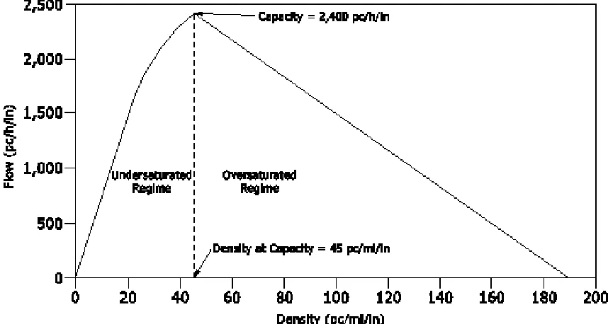
Figure 2.3 Example fundamental flow-density diagram (Highway Capacity Manual2016). 10
Figure 2.4 Dynamic Traffic Assignment representation of a network showing source and
sink nodes added. Flow conservation can be preserved at these nodes. . . 14 Figure 2.5 . . . 24
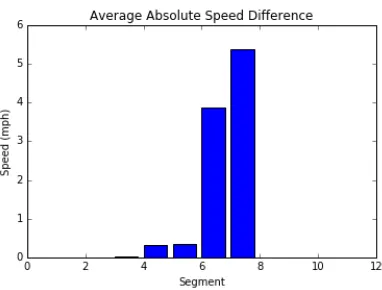
Figure 2.6 Average absolute speed difference between solutions for each methodology
for each segment along the facility over the course of the three hour study period . . . 25 Figure 2.7 Geometry of the I-40 example facility. . . 27
Figure 2.8 Speed contours for the I-40 facility before and after ramp metering. . . 29
Figure 3.1 Example of a basic facility modeled in the HCM freeway facilities model
(Highway Capacity Manual2016). . . 33
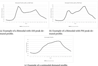
Figure 3.2 Examples of well-known behavior exhibited in daily demand profiles (NCDOT,
2016). . . 36
Figure 3.3 Core freeway analysis calibration framework in the 6th edition of the HCM
(Highway Capacity Manual2016). . . 37
Figure 3.4 National default hourly demand profiles for weekdays and weekends on urban
and rural interstates. . . 38 Figure 3.5 Flow chart detailing the process of a genetic algorithm. . . 42
Figure 3.6 Example of an input demand profile shape with a 15% search interval specified
around it. . . 43
Figure 3.7 Visual example of the skew normal and skew Cauchy distributions. Both
distributions are generated for a meanµof 0 and a standard deviationσof 1. 46
Figure 3.8 Example demonstrating the encoding of ann-distribution candidate profile
into a binary string. . . 48 Figure 3.9 Full mixture distribution encoding example. . . 49 Figure 3.10 Visualization of the three crossover strategies. . . 52 Figure 3.11 Plotted results for matching the six unimodal subtypes. The true profile shape
is represented by the red line, and the computed profile is shown as the blue dashed line. . . 57 Figure 3.12 Bimodal with PM peak known profiles (NCDOT, 2016). The red line represents
the true profile, the blue dashed line shows the computed profile, and the green lines provide a 10% relaxation bandwidth of the profile. . . 58 Figure 3.13 Geometry of the simple example facility. The lane drop in segment 26 provides
a bottleneck for the facility that creates two congested regimes. . . 59 Figure 3.14 Bimodal with AM peak 25th percentile demand profile (NCDOT, 2016). . . 59 Figure 3.15 Speed contour predicted by the HCM analysis for the contrived ground truth
Figure 3.16 Demand profile comparison and speed contour of the initial guess demand volume inputs. . . 61 Figure 3.17 Contour highlighting the speed differences between the GA run with the
lowest total speed error and the target data set. White cells represent minimal speed errors, while red cells indicate larger speed errors. . . 63 Figure 3.18 Comparison of profiles generated by the best and worst calibration of the
GA framework. The true profile is represented by the blue dotted line, and the initial incorrect profile is shown as an orange dotted line. The black line represents the profile as calibrated by the GA framework. . . 64 Figure 3.19 Side by side comparison of the target speeds (left) and the speeds predicted
by the best GA run (right). . . 66 Figure 3.20 Comparison of profiles generated by the best and worst calibration of the GA
framework. The true profile is represented by the blue dotted line and the black line represents the profile as estimated by the GA framework. . . 66 Figure 3.21 Geometry and target speed data for the I-540 WB case study. . . 68 Figure 3.22 Speed contour predicted by the HCM analysis for the initial demand assignment. 69 Figure 3.23 Predicted speed contour of the profile-based demand calibration run with
the lowest total speed error. . . 72 Figure 3.24 Predicted speed contour of the demand estimation run with the lowest total
speed error. . . 75
Figure 4.1 Core freeway analysis calibration framework in the 6th edition of the HCM
(Highway Capacity Manual2016). . . 80
Figure 4.2 Effects of different pre-breakdown bottleneck capacities (Highway Capacity
Manual2016). . . 84
Figure 4.3 Effects of two different capacity drop percentagesα1andα2(Highway
Capac-ity Manual2016). . . 85
Figure 4.4 Effects of varying jam density values Kj,1and Kj,2on the volume density
diagram (Highway Capacity Manual2016). . . 86
Figure 4.5 High-level process flow of the unified two-stage calibration process. . . 89
Figure 4.6 Example of encoding three pre-breakdown CAFs and the facility-wide jam
density into binary strings based on the values of Table 4.2. . . 92
Figure 4.7 Demonstration of three common crossover operators. . . 94
Figure 4.8 HCM segmentation of the 14.5 mile section of I-540 westbound near Raleigh,
NC. . . 94
Figure 4.9 Speeds obtained from the real-world sensor data for Tuesday August 19th
2014 (top) and those initially predicted by the FREEVAL computational engine for the uncalibrated I-540 case study facility. . . 96 Figure 4.10 Comparison of the target speed contour (top) and the speed contour as
pre-dicted by the partially calibrated facility after Phase 1. . . 100 Figure 4.11 Comparison of target speed contour (top) and the speed contour as predicted
by the calibrated facility after Phase 2. . . 104 Figure 4.12 Chart showing the set of pre-breakdown CAFs for all segments of the facility
as estimated during the Phase 2 calibration process. . . 106
CHAPTER
1
INTRODUCTION
The 2015 Urban Mobility Scorecard reports that drivers nationwide suffer through more than 7 billion hours of delay per year due to traffic congestion, costing the nation as a whole at least
$160 billion dollars and wasting 3 billion gallons of fuel.1When pairing this knowledge with the
frustration of sitting in bumper to bumper traffic, few would argue that improving the nation’s transportation systems is not a massively important endeavor. There are many avenues through which improvements can be made, but one of the most obvious areas centers on reducing congestion and delay on freeways. In a perfect world with an unlimited budget, all delay could be eliminated by simply increasing the capacity of freeways far beyond the expected traffic demands. However, in reality, funding for infrastructure projects is often very limited, and great care must be taken to ensure that the projects that are undertaken are well planned and carried out efficiently.
A variety of planning and analysis tools are used to aid in project planning and execution. The Highway Capacity Manual is one such tool whose goal is to provide methodologies and algorithms
to “assess the traffic and environmental effects of highway projects."2In particular, the manual
includes afreeway facilitiesmethodology rooted in the hydrodynamic theory of traffic flow which
has been shown to be an effective approach for planning and operational analysis. Despite being
1Schrank,David, et al. “2015 Urban Mobility Scorecard." (2015). https://mobility.tamu.edu/ums/
2Highway Capacity Manual 6th Edition: A Guide for Multimodal Mobility Analysis. Transportation Research Board,
Washington, D.C., 2016.
widely used, little has been done to take advantage optimization techniques in conjunction with the methodology. Incorporating optimization techniques can greatly expand the scope of the analysis and provide novel approaches for a number of new planning, operational, and congestion man-agement applications. Additionally, in order for these types of analyses to be useful, they must be conducted on models that have first been calibrated to accurately represent observed real-world conditions. The model calibration process, which represents a major barrier to entry for use of the methodology, can also be vastly improved with optimization techniques by providing a new automated framework to replace the current arduous manual procedure. Consequently, the goal of the work presented is to explore improvements to the existing methodology through the use of both classical and metaheuristic optimization approaches. The work is presented as three chapters, with each constituting an individual paper.
Chapter 2 utilizes linear programming to provide a new optimization framework for conducting congestion analysis with the methodology. The framework is intended for use with calibrated models and works with known inputs and parameters to improve the performance of a specific aspect of the system, or the system performance as a whole. The new framework is created by reformulating the
analyticaloversaturatedmodels as a set of linear constraints. These constraints can then be paired
with a variety of objective functions that tailor the framework for use in congestion management approaches. In this context, the methodology emulates a dynamic traffic assignment model, and the system optimal approach can be used for a number of different applications. Two specific applications are demonstrated in the chapter. First, an analysis that computes an optimal spreading of peak demand is presented. This approach uses an objective function that minimizes the total delay of the system while maintaining the core node-flow relationships of the model. Next, a system-optimal ramp metering approach is presented that relaxes flow constraints loading the system at on-ramps in order to improve the overall performance.
The following two chapters take a step back and address the process of calibrating a core facility model. The calibration process is a foundational aspect of using the methodology and a critical step of model creation that precedes all conducted analyses. Model calibration is essential because any analysis that uses the method, including that as proposed above, hinges on the core model correctly representing daily recurring congestion conditions. In fact, modeling existing real-world conditions for a single representative day is the first step for using the methodology in conducting reliability and active traffic management analyses. This requirement necessitates that every model must be calibrated to match a set of target real-world conditions. The manual’s current guidance concerning calibration is very limited, and the process often presents a major barrier to entry for the methodology.
large number of inputs, with even moderate sized models requiring the input and adjustment of thousands of individual parameters. Further, many of the critical inputs are difficult to measure under real-world conditions. Calibration of both input demand volumes and capacity parameters is vitally important as the driving force of the methodology is the relationship between demand volumes and segment throughput capacities. However, vehicle demand volumes are largely un-known under real world conditions and are essentially impossible to measure when traffic flow is congested. The manual does provide default estimates for the key capacity parameters, but these should ideally be adjusted in conjunction with demand volumes for each specific facility location. A genetic algorithm metaheuristic framework is first developed in Chapter 3 to address the challenges of demand estimation in the context of model calibration. Two encoding approaches for the problem are proposed based on the quality of available data. One approach makes use of existing knowledge of hourly demand profiles, while the second utilizes mixture distributions of random variables in order to allocate demand over the course of a study period when the behavior is unknown. A genetic algorithm is then used to manipulate the individual demand inputs to find a set of overall volumes that minimizes the errors between predicted outputs and a set of target real-world performance measures (e.g., segment speeds). The effectiveness of the approach is tested on both an ideal facility with known demands and a single bottleneck, as well as a case study in Raleigh, NC, where the underlying demands are unknown.
Chapter 4 expands upon the demand estimation approach by adding three key capacity parame-ters into the existing calibration framework. New genetic encodings for the inputs are developed that allow the metaheuristic to consider pre-breakdown capacity adjustments, the queue discharge flow rate, and the facility-wide jam density alongside demand volumes. These three capacity parameters are important to incorporate as each controls aspects of breakdown occurrence, queue formation and recovery speeds, and overall queue size in a unique way. The resulting framework consists of a two-phase calibration process. During the first phase, the GA adjusts demand volumes and the queue discharge rate, while at the second phase the GA manipulates the jam density and bottleneck segment pre-breakdown capacity adjustments. Further, unlike the initial work of Chapter 3, this expanded approach utilizes an updated objective function that considers errors in both facility travel times and individual segment speeds. The effectiveness of the framework is once again tested on the North Carolina case study facility, and an analysis of the calibration resulting from the metaheuristic approach is presented.
CHAPTER
2
A LINEAR PROGRAMMING
FORMULATION FOR CONGESTED
FREEWAY FACILITIES
2.1
Introduction and Motivation
The Highway Capacity Manual (HCM) was first published in 1950 with the goal to provide method-ologies and algorithms to “assess the traffic and environmental effects of highway projects" (Highway Capacity Manual2016). Of the manual’s many approaches, this research focuses on thefreeway facilitiesmethodology, which was first introduced into the manual in 2000. The HCM freeway facilities methodology is a macroscopic simulation technique and computational procedure to calculate flows and speeds on an extended length of freeway. The driving force of the methodology is the relationship between three key quantities: the demand flow rate (demand input), segment capacities, and the actual flow rate (volume served). The analysis is divided into two operational
regimes. A facility is considered to beundersaturatedwhen the demand input never exceeds the
The oversaturated methodology is based on the Cell Transmission Model (CTM), which is rooted in the hydrodynamic theory of traffic flow (Daganzo, 1994). The oversaturated methodology expands on the core CTM methodology by introducing additional relationships to better capture congestion dynamics, as well as capabilities to track the horizontal propagation of vehicle queues. The associated
computational procedure for theoversaturatedmethodology is presented as an iterative method
that progresses in a “forward" manner across both the spatial and temporal dimensions of an analysis. While this formulation is adequate for a direct application of the methodology, its use is very limited for any additional analysis of the core flow relationships.
The limitations of the procedure stem in part from the nature of the relationship between demand, capacity, and volume served. For each flow relationship, volume served is specified to be the exact minimum of demand and any constraints on throughput capacity. The “exactness" here serves a number of important purposes, including helping the analysis to approximate a “first-in, first-out" (FIFO) condition, as well as a User Optimum (UO) system utilization property. However, using just the minimum of a set of values at each step effectively funnels out and discards information that may still be relevant for additional analysis. The discarded information is potentially valuable for reconstructing inputs from outputs, and can be instrumental for sensitivity analysis of facility performance under varying conditions.
The iterative nature of the formulation also comes with its own set of inherent limitations.
Each facility analyzed in the methodology is broken down spatially into connectedsegments, and
the group of segments is analyzed over the course of a study period consisting of consecutive 15-minute analysis periods. Within each analysis period, the procedure iterates downstream along the facility (i.e., in the direction of traffic flow), computing the congestion conditions at each segment. However, as currently constructed, at each computational step the procedure can only make use of information known from the current or previous steps. This restriction substantially limits the usefulness of the methodology as part of a framework for system level optimization approaches.
This paper presents formal mathematical programming techniques that provide a novel linear programming analysis framework for the HCM’s freeway facilities methodology. This new framework helps to addresses many of the limitations of the current computational procedure. Each of the key flow relationships of the methodology is examined and reformulated as a set of linear constraints. By defining the relationships in this manner, the methodology is opened up beyond just the basic direct application and analysis allowed by the iterative approach. The type of sensitivity analysis allowed by linear programming can provide new insight into the relationships between inputs, outputs, and intermediate flow quantities that can help to better understand and predict facility performance. Further, the framework allows for optimization approaches that can be used for facility operational and design analysis, as well as for the development of new traffic management techniques.
2.2
Overview of the HCM Freeway Facilities Methodology
The HCM defines afreeway facilityas an extended length of freeway composed of continuously
connected basic freeway, weaving, merge, and diverge segments (Highway Capacity Manual2016).
In the context of the methodology, a facility is generally a 9-12 mile portion of a single freeway as opposed to an interconnected network of freeways. For a typical freeway facilities analysis, a study period falling within a 24-hour time period is specified and divided into 15 minute analysis periods.
In order to conduct traffic flow analysis, the HCM provides four core methodologies that can be used to analyze each type of segment on a individual basis. While these methodologies can be used for some operational and design analyses, they are inherently limited in scope as they cannot capture conditions that extend beyond the boundaries of the uniform segments. This is problematic as most analysis of interest involves traffic congestion and the formation of vehicle queues that can extend far beyond the allowable length of a single segment type. In order to accurately capture these types of conditions, the freeway facilities methodology was developed to unite and extend the four
core segment methodologies (Highway Capacity Manual2016).
For both the freeway facility and the segment methodologies, the analysis revolves around the
relationship between thedemand flow rateand theactual flow rate. The demand flow rate, or
input demand, is defined to be the number of vehicles that wish to traverse the facility or segment during a given time period. The actual flow rate, or volume served, is the number of vehicles that are actually able to move through the segment after accounting for maximum link capacities and related congestion conditions. In the context of these two quantities, the methodologies treat the flow through each segment as the minimum of the desired input and the available output.
When the input demand is less than the available capacity, the analysis is straightforward. The underlying hydrodynamic theory allows flow-density diagrams and speed-flow equations to be used to estimate segment and facility performance measures. Additionally, because all demand is being met in this case, the segments can be analyzed individually as their performance conditions are effectively independent. However, at times where the demand flow rate is greater than the allowable actual flow rate, the analysis can change drastically. In the event that demand exceeds capacity,
and abottleneckand resulting flow breakdown occur, the individual segment methodologies can
no longer provide accurate results. The effects of unserved demand can extend upstream to addi-tional segments, and the effects of restricted demand rates may be felt on flows downstream of the bottleneck.
can be fully captured in the spatial and temporal domain of the system. Some methods resort to tracking queues “vertically" on a single segment, but this solution is far from desirable when dealing with situations involving large queues that span multiple segments. The HCM’s freeway facilities methodology provides a solution to this issue by allowing a facility to be analyzed as a whole. This increased spatial extent can be used to accurately model the accumulation and upstream propagation of queues. Allowing queues to be tracked “horizontally" reflects real world behavior. Further, when the extent of the spatial domain is chosen well, even the effects of a bottleneck on downstream flow can also be modeled.
2.2.1 The Oversaturated Equations
The freeway facilities methodology considers a facility at all times to be in one of two states. Due to the existence of these two conditions, the freeway facilities methodology relies on two connected sets of equations for its analysis. The first is the undersaturated method, which utilizes the individual segment methodologies to analyze a facility. The second algorithm is the oversaturated method, which is invoked as soon as demand exceeds capacity in at least one segment along the facility.
Figure 2.1 Diagram of the node-segment relationship. (Source: (Highway Capacity Manual2016))
The oversaturated method introduces more complex flow and queuing equations in an effort to capture the congestion dynamics that may arise. The method also instantaneously increases the computational resolution by breaking each 15 minute analysis period into sixty 15 second time steps and slightly adjusting the spatial domain. Instead of just analyzing the conditions at each segment, the facility is viewed as a set of nodes and segments as is shown in Figure 2.1. Flows are computed at each node, and segments are used to track stored vehicles and flow densities. At its simplest, the flow through each node is the minimum of input demand and segment capacity. The presence of congestion and queuing can introduce new limits on the output available at a node. These new restrictions can arise from turbulence due to cars entering a congested mainline from an on-ramp, as well as due to the build up of queues during previous time steps. The oversaturated methodology accounts for these situations by introducing new quantities into the flow relationships
defined at each node type. These new relationships are discussed in Section 2.4.
The oversaturated equations evaluate the facility by computing flows for each node, starting at the first upstream node and moving down the facility. Traffic demand enters the facility at the
upstreammainlinesegment, and flows down the facility until it exits either at adiverge(off-ramp)
segment or at the end of the facility. In addition to the demand entering the facility at the upstream
segment, demand can enter atmerge(on-ramp) segments provided that the segment has enough
capacity to contain both flows. Flows at each node consist of three quantities, mainline flow (MF), on-ramp flow (ONRF), and off-ramp flow (OFRF). Segment flows (SF) are calculated for each inter-mediate segment between every pair of nodes. Figure 2.2 shows how mainline and segment flows interact at merge and diverge segments.
Figure 2.2 Example of the mainline flow (MF) and segment flow (SF) calculations with on-ramps and off-ramps.
For this research, the assumption is made that computation for an entire study period can just be confined to the set of oversaturated equations. This assumption is made for two reasons. First, it is possible to analyze undersaturated conditions using the oversaturated equations with a similar degree of accuracy. Second, analysis periods in which a facility is undersaturated have limited usefulness. As such, this research can assume study periods are almost completely restricted to times where the facility is oversaturated. All that is required is that the study period include a small number of undersaturated “warmup" and “cooldown" periods at the beginning and the end of the analysis. These ensure that the congestion and queues have time to build correctly and fully dissipate, and can generally consist of a single undersaturated period at both the beginning and end of a study period.
2.3
Literature Review
and extensions and updates to the Cell Transmission Model (CTM). Most of the work presented in the following sections is built either on top of the CTM or a simplified set of flow and traffic assignment equations.
2.3.1 Overview of Dynamic Traffic Assignment and the Cell Transmission Model
An important analysis technique used in planning and evaluating freeway transportation networks is Dynamic Traffic Assignment (DTA). DTA seeks to model “time-varying network and demand interaction using a behaviorally sound approach" (Chiu et al., 2011). This research is primarily
interested in a subset of DTA consisting of equilibrium-seekingmesoscopicmodels, i.e., models
whose resolution falls between microscopic and macroscopic models, but make use of properties of both.
DTA models are often used to evaluate travel times and costs of network performance by mod-eling them as optimization problems. In these formulations, travel time and cost become the objectives to be minimized and are subject to flow conservation and traffic assignment constraints. Throughout the literature reviewed, two different traffic assignment conditions were generally used for the DTA formulations. The first and simpler of the two conditions is the System Optimum (SO) condition. Under SO assignment, the goal is to minimize the travel time or cost of the system as a whole (Ziliaskopoulos, 2000). The second condition, User Equilibrium (UE) or User Optimum (UO)
assignment, differs from this in that each individual driver seeks to minimize his/her travel time,
even if it comes at the cost of total system performance (Ukkusuri & Waller, 2008). This dynamic can be more difficult to capture in mathematical models, but is generally thought of to be a more realistic representation. It should be noted that under free flow conditions with little to no congestion, the two conditions will converge to the same answer, but when congestion is high, the optimal solutions can differ greatly. An in depth survey on DTA is given by Chiu et al. (2011).
One of the more widely used DTA models is the Cell Transmission Model (CTM), which was first proposed by Carlos Daganzo (1994). The CTM primarily consists of a set of difference equations that simulate traffic flow on highways and use shockwaves to model the backward (upstream) propagation of traffic congestion. The equations are presented as a discrete approximation of the differential equations proposed by Lighthill, Witham, and Richards (Lighthill & Whitham, 1955a,b; Richards, 1956). These original differential equations (often referred to as the LWR equations) were developed by applying hydrodynamic flow theory to traffic flow and analytically account for important concepts such as the Flow-Density diagram (Figure 2.3) and the shockwave propagation of congestion. In his initial paper, Daganzo asserts that the CTM is the discrete equivalent of the underlying hydrodynamic theory. The equations that make up the CTM allow for four distinct
inputs: the free flow speed (FFS) of the highway, the maximum flow in a cell (segment capacity), the jam density, and the wave speed of the propagation shockwaves. Work was later done by Daganzo (1995) to expand the model to represent traffic networks by allowing for basic, merge (on-ramp), and diverge (off-ramp) segments to be represented in the equations. Due to its accuracy (as shown in (Lin & Ahanotu, 1995; Smilowitz & Daganzo, 1999)) and relative computational simplicity, vast amounts of research have been conducted to expand the core methodology of the CTM.
Figure 2.3 Example fundamental flow-density diagram (Highway Capacity Manual2016).
2.3.2 Optimization Extensions to the Core CTM Formulation
Travis Waller & Ziliaskopoulos (2006) first proposed a combinatorial optimization approach (as opposed to mathematical programming), while later Ukkusuri & Waller (2008) directly extended the CTM linear programming formulation to account for UE conditions. In their work, they also compared the effect of the two route assignment conditions (SO and UE) on solutions for sample TNDP problems. Han et al. (2011) further built on the formulation making use of complementarity theory to improve the calculation of travel time estimates and capture multiple user classes with elastic demands. Active Traffic Management (ATM) techniques such as dynamic congestion pricing for tolls have also been proposed based on sensitivity and dual variable analysis allowed by the linear programming formulations (Lin et al., 2011).
In order to model the CTM as a pure linear program, Ziliaskopoulos (2000) used the simplifying assumption that the minimum relationship between flow and capacity could be represented as a set of “less-than" inequality constraints on link flow. However, this assumption does not guarantee
that the assigned quantity is truly the minimum of the values, i.e.,x ≤y,x ≤z does not imply
x=min{y,z}. This can lead to an issue known as thevehicle-holdingorholding-backproblem.
An overview of theholding-backproblem as well as a survey of the work done to account for it
was compiled by Doan & Ukkusuri (2012). Lo (2001) proposed accounting for this nonlinearity by incorporating integer linear constraints that effectively turn sets of constraints on or off, though the work was mostly investigated for its use in signal control applications. In a similar vein, Tampère & Immers (2007) proposed the use of the Heaviside function for the approach. Zheng & Chiu (2011) addressed the issue by proving that the single destination system optimal dynamic traffic assignment (SD SO-DTA) problem is equivalent to the earliest arrival flow (EAF) network problem, and developed a network flow algorithm that eliminated vehicle holding in basic and merge segments (but not necessarily for diverge segments).
Doan & Ukkusuri (2012) presented multiple formulations to completely remove vehicle-holding under SO routing for problems with multiple destinations. The removal of vehicle-holding was achieved by using complementarity constraints and converting them to a nonlinear programming model, as well as by incorporating mixed integer programming (MIP) techniques. Next, Ukkusuri et al. (2012) extended the techniques to handle the UE conditions. Unfortunately, each of these formulations requires assumptions that may not accurately reflect realistic conditions, and in addition still contain some nonlinearities or non-convexities (Zhu & Ukkusuri, 2013). Further, in all of the previously mentioned papers the authors acknowledge that the formulations are still impractical for larger and more realistic sizes of networks.
Another linear complementarity approach was developed by Zhong et al. (2013) in order to
better deal with the nonlineararity of the state jump conditions and hard nonlinearminfunctions.
The proposed formulation readily extends to both DTA and TNDP analysis, and while not as
putationally efficient as pure LP formulations, it benefits from the existing work done on linear complementarity problems (LCP) (Hu et al., 2012). More recently, Zhu & Ukkusuri (2013) were able to develop a pure linear programming solution to the vehicle-holding problem for the SD SO-DTA problem by introducing an easily computable penalty function into the formulation. Sun et al. (2014) extended this to incorporate demand uncertainty and developed an adjustable robust optimization (ARO) linear programming formulation.
2.3.3 CTM Formulations and ATM Analysis
The CTM formulation and its extensions have also been used to tune ATM strategies. Gomes & Horowitz (2006) developed the Asymmetric Cell Transmission Model (ACTM) to compute optimal ramp metering rates. While the ACTM formulation remains nonlinear, the authors proved sufficient conditions under which the globally optimal solution could be found through the use of a single linear program. Unfortunately, these sufficiency conditions were rather constrictive, and often highly unrealistic of true freeway conditions. Finding a lack of in-depth theoretical results concerning the
CTM/MCTM, Gomes et al. (2008) further investigated the properties of congested and uncongested
equilibria for the model and interpreted the findings with respect to the effectiveness of ramp metering strategies. The authors found that optimally computed ramp metering strategies can reduce congestion and travel time on freeways, and that the strategies do more than just move the congestion to on-ramps. A dynamic on-line method to determine Variable Speed Limits (VSL) has been proposed by Li et al. (2014), with benefits stemming from the low computational cost of the CTM vs the more complex existing VSL algorithms.
2.3.4 Overview the Transportation Network Design Problems (TNDP)
2009).
Due to the interplay between the equilibrium constraints and the multiple objective functions, single level TNDP formulations are generally nonconvex and nonlinear. These types of problems are known to be at least NP hard (Zeng & Mouskos, 1997). To regain some linearity, TNDP is often
formulated as abilevel program, i.e., one with an upper level and a lower level objective function.
Despite the inherent difficulty in finding a solution for formulations such as these, it is still impor-tant that at least a near globally optimum solution be found. As such, heuristic algorithms have often been found to be the best choice to efficiently seek an optimal or near-optimal solution. In recent years, much research has been conducted into the use of metaheuristic techniques such as genetic algorithms (GA), simulated annealing (SA), and tabu search for extending and solving TNDP formulations (Delbem et al., 2012; Juan et al., 2012; Karoonsoontawong & Waller, 2006; Luathep et al., 2011; Mudchanatongsuk et al., 2008; Xu et al., 2009; Zeng & Mouskos, 1997).
2.4
Formulation of Methodology as Dynamic Traffic Assignment
With the exception of the minimum and maximum functions, the majority of the key flow and asso-ciated relationships of the HCM’s oversaturated model are linear. Thus, so long as those functions can be approximated linearly, this allows the methodology to be incorporated into classical linear optimization approaches. A minimum or maximum of a set of values can easily be approximated through a group of linear inequalities, which can then serve as constraints in a linear optimization model. In general, this falls under the umbrella of linear programming, which consists of a linear objective function that is minimized (or maximized) subject to a set of linear inequality and equality constraints. For the purposes of this work, any number of objective functions can be chosen, and it will largely serve as a way to tailor the model for the various applications. The is because the crux of the model is truly found in the constraints. The relationships laid out therein define and govern the flows along the facility such that they are consistent with the oversaturated methodology. In this way, the formulation can be thought of as a dynamic traffic assignment (DTA) model.
Further, through the addition of two “dummy" nodes to the model, a freeway facility can be thought of as being a single origin - single destination network. These two added nodes serve as source and sink nodes for the demand desiring to use traverse the network. In this way, a freeway facility can be thought of as having a single origin and a single destination. However these dummy nodes are never explicitly used in any computations. Figure 2.4 shows a facility with one on-ramp, one weave, and one off-ramp and the corresponding single origin - single destination DTA network representation.
As stated earlier, DTA models generally fall into two types: system optimal (SO) or user optimal
Figure 2.4 Dynamic Traffic Assignment representation of a network showing source and sink nodes added. Flow conservation can be preserved at these nodes.
(UO) (Ukkusuri & Waller, 2008). Treating the minimum functions as a group of “less-than" constraints inherently leads to the SO condition as the exact flows may not be forced through each node when it is detrimental to the system performance as it defined in the objective function. The primary challenge of modeling the freeway facilities method of the HCM in an optimization framework comes from exactly this. Depending on the choice of objective function, simply using inequalities
can lead to the phenomenon ofholding-backflows. Holding-back flows are a commonly arising issue
in macroscopic dynamic traffic assignment, and the resulting model will generally be considered to be a system optimal model. While this type of model is not necessarily as realistic as a user optimal model, it still provides many useful insights for both planning and operational purposes.
It is important to note that the model proposed in the following sections differs from the HCM’s computational procedure in a number of ways. While both operate on a known set of demand and capacity inputs to compute the resulting flows and performance of the system, the proposed formu-lation approaches the methodology in a fundamentally different way than the current framework in order to provide new avenues for analysis of the flow relationships. Specifically, the computational procedure seeks to build a solution by analyzing facility conditions in an iterative manner. On the other hand, the use of linear programming allows us to define the desired properties of a solution through a set of constraints. Solving the LP then allows us to seek solutions with those properties that are optimal in regards to a specified set of metrics.
preserving this condition under high levels of congestion — an issue discussed in more detail in Section 2.4.4. This model also is limited in its ability to enforce a UO condition. As discussed in the literature review, work has been done to implement the UO condition for similar models, and much of that work can be directly applied to the model. However, for the purposes of this paper, the model is never assumed to enforce the UO condition.
Table 2.1 Summary of key variables and parameters of the oversaturated methodology.
Symbol Definition
Indices
NS
Set of indices indicating the node,i=1, ...,|NS|. The number of nodes is
one greater than the number of segments. Segmenti refers to the segment
immediately downstream from nodei.
S Set of indices indicating the time step of the current period,t =1, ..,|S|.
P Set of indices indicating the current analysis period,p=1, ...,|P|.
˜
N Index set of the on-ramp segments of a facility, ˜N⊂NS
˜
F Index set of the off-ramp segments of a facility, ˜F ⊂NS
Segment Variables
NVi,t,p Number of vehicles on a segmenti, in stept, for periodp.
UVi,t,p
Unserved vehicles: the additional number of vehicles stored in Segmenti at the
end of time stept in intervalp due to a downstream bottleneck.
SFi,t,p Segment flow out of segmenti during stept in intervalp.
S Ci,p Capacity of segmenti in analysis periodp.
KBi,p Background density of segmentiduring analysis periodp.
K J Jam density - the maximum per lane density allowed on a segment.
K C Ideal Density - the per lane density of a segment operating at capacity
Li Length of segmenti.
NL
i Number of lanes in segmenti.
Node Variables
MIi,t,p Desired mainline input flow into nodeiduring time stept in periodp.
MFi,t,p Actual mainline flow rate leaving nodei during time stept in periodp.
ONRFi,t,p Actual ramp flow rate that can cross on-ramp nodei during stept in periodp.
ONRQi,t,p Queue due to unmet on-ramp demand at nodei during stept in periodp.
OFRFi,t,p Actual flow that can exit at off-ramp nodei during time stept in periodp.
There are three principal segment variables that are used in order to track and assess the flow of vehicles on a facility. The first is the number of vehiclesNVi,t,pon particular segmentiin time step
t, in time periodp. The second is the number of unserved vehiclesUVi,t,pon particular segment
iin time stept, in time periodp. Lastly, the variableSFi,t,pis defined to be the segment flow for
a segmenti, in time stept for time periodp. Almost all traditional performance measures for
the analysis can be calculated using some combination of these three values in combination with the underlying facility characteristics. Additionally, there exist three node flow variables that track the mainline flow, on-ramp flow, and off-ramp flow. These are denotedMFi,t,p,ONRFi,t,p, and
OFRFi,t,p, respectively. Table 2.1 provides a summary of the initial model variables.
2.4.1 Flow Conservation
Since the underlying principles of the methodology are based on hydrodynamic theory, one of the first relationships that should be considered is one that ensures a “conservation of flow" (Daganzo, 1994, 1995). The property is implicitly present in the iterative procedure, but requires an explicit constraint in the linear programming framework. Equation 2.1 achieves this and states that all demand that enters the facility at the first upstream segment or at an on-ramp, must also exit the facility at the final downstream mainline segment or an off-ramp. Consequently, there is an implicit assumption that the length of the study period chosen for the analysis allows the flows to fully discharge, but equation 2.1 can be relaxed to an inequality to allow queues to persist through the end of the study period.
|S| X
t=1
|P| X
p=1
MF0,t,p+
X
i∈N˜
ONRFi,t,p=
|S| X
t=1
|P| X
P=1
MFN S,t,p+
X
i∈F˜
OFRFi,t,p (2.1)
There are four equations in the HCM related to flow conservation that can be directly incorpo-rated into the linear programming model. Equation 2.2 initializes each segment at the beginning of each analysis period by defining the minimum number of vehicles that will be on a segment at any point int time based on the underlying demand. Equation 2.3 states that the number of vehicles on a segment is equal to the number of vehicles on the segment at the previous time step, plus the input
from the upstream node (i), and minus the output at the downstream node (i+1). A new constraint
is added here to ensure that the number of vehicles on a segment at any step never exceeds the
maximum allowed by the pre-specified jam densityKJ. Equation 2.5 serves to track the growth and
dissipation of any vehicle queues that may form in the analysis. The constraint defines the number of unserved vehicles to be any vehicles on segment exceeding the normal operating background density, a value computed from demand inputs. Lastly, equation 2.6 defines the segment flow, which can be used to compute the speed at a segment.
following sections will present each flow sub-problem in a declarative manner that approximates the relationships as they are defined in the HCM.
NVi,0,p=KBi,pLi+UVi,S,p−1 ∀i∈NS,p∈P (2.2)
NVi,t,p=NVi,t−1,p+MFi,t,p+ONRFi,t,p−MFi+1,t,p−OFRFi+1,t,p ∀i∈NS, t ∈S p∈P (2.3)
NVi,t,p≤NiLLiKJ ∀i∈NS, t ∈S p∈P (2.4)
UVi,t,p=MIi+1,t,p−MFi+1,t,p ∀i∈NS, t ∈S p∈P (2.5)
SFi,t,p=MFi+1,t,p+OFRFi+1,t,p ∀i∈NS, t ∈S p∈P (2.6)
2.4.2 Mainline Flow
The formulation of the mainline flow relationship presents the biggest differences between the HCM oversaturated methodology and the CTM. Consequently, it is also the main area in which this model deviates from the SO-DTA formulation proposed by Zilliaskopolous. In addition to a segment’s capacity, the HCM introduces three new limits on mainline flow output in order to capture additional congestion dynamics. These three values are referred to as Mainline Outputs 1, 2, and 3, respectively. The following set of linear equalities and inequalities approximates the mainline flow relationship as it is defined in the HCM.
MIi,t,p=MFi−1,t,p+ONRFi−1,t,p−OFRFi,t,p+UVi,1,t,p ∀i∈NS, t ∈S,p∈P (2.7)
MFi,t,p≤MIi,t,p ∀i∈NS, t ∈S,p∈P (2.8)
MFi,t,p≤SCi,t,p ∀i∈NS, t ∈S,p∈P (2.9)
MFi,t,p≤SCi−1,t,p ∀i∈NS, t ∈S,p∈P (2.10)
MFi,t,p≤MO1i,t,p ∀i∈NS, t ∈S,p∈P (2.11)
MFi,t,p≤MO2i,t,p ∀i∈NS, t ∈S,p∈P (2.12)
MFi,t,p≤MO3i,t,p ∀i∈NS, t ∈S,p∈P (2.13)
Equation 2.7 defines the desired mainline input into the node, and equations 2.8 – 2.13 limit the flow to be less than the desired input at the node and available throughput of the node. Each of the
three mainline outputs serves to limit throughput in a unique way. The first, denotedMO1, accounts
for limits on node output based on turbulence due to merging on-ramp flows. This relationship is defined as the minimum of three values in the HCM, and can be approximated by the following
three inequalities.
MO1i,t,p≤SCi,t,p−ONRFi,t,p (2.14)
MO1i,t,p≤MO2i,t−1,p (2.15)
MO1i,t,p≤MO3i,t−1,p (2.16)
Mainline Output 2 (MO2) serves to limit node output due to queue accumulation from a
down-stream bottleneck. In the HCM methodology, this value is computed by first estimating the maximum
densityKQallowed on a segment based on the size of its queue, and limiting the flow entering the
segment from the node to be no greater than that which would push the segment to the maximum allowed density. However, because the HCM procedure is iterative, queue size for the segment
at the current step is unknown at that point in the computations, soKQmust be estimated from
conditions the previous time step. This estimation is made by computing the maximum density
allowed by the flow rate, utilizing the jam capacityKJ, the ideal capacityKC, and the decreasing
linear relationship of the flow density diagram that exists when density is greater than capacity (see Figure 2.1). Equations 2.17 and 2.18 show these relationships.
KQi,t,p=KJ−
KJ−KC SCi,p ∗
SFi,t−1,p (2.17)
MO2i,t,p=SFi,t−1,p−ONRFi,t,p+KQi,t,p∗Li−NVi,t−1,p (2.18)
Since our LP model lacks this restriction of known information, it is possible to reformulate this relationship through an alternative, and arguably more accurate, set of equations. First, it must be
noted that a key assumption for the HCM procedure for calculatingKQis that a queue exists on the
downstream segment, which indicates that flow is on the right side of the flow density relationship. Otherwise, the same value for flow can correspond to two different densities. Hence a check on the
size ofUV at the downstream segment is required, which necessitates the use of integer variables
to implement correctly. To avoid this, we can invert the relationship, and the maximum allowable
segment flow for a given segment density can be used to the same effect. Further, sinceMO2should
only limit flow in the presence of a queue, we can simply extend the linear relationship of the right side of the flow-density diagram to compute the maximum allowable segment flow at any density.
Once the maximum allowable segment flow has been determined,MO2is simply that value minus
2.19 and 2.20.
ASFi,t,p=
[KJ∗NiL]−NVi,t,p+NVi,t−1,P 2∗Li
∗ SCi,p
NiL∗(KJ−KC) (2.19)
MO2=ASFi,t,p−ONRFi,t,p (2.20)
The final limit on mainline output (M O3) models the effects of queue dissipation of
front-clearing queues. A queue is considered to be “front-front-clearing" when the queue density decreases while the rear position of the queue remains unchanged. Modeling this behavior requires a linear
estimation of the recovery wave speed1ws
i,pbased on capacity as well as on known ideal and jam
densities. The recovery speed is then translated to the wave travel time2wtti,pbased on the length
of the segment being analyzed. A more detailed explanation of front-clearing queues can be found
in theHighway Capacity Manual(2016). TheMO3relationship is presented as a single minimum
statement in the HCM methodology and can thus be directly approximated using a set of linear inequalities as shown in equations 2.21 - 2.25.
MO3i,t,p≤MO1i+1,t−wtt,p−ONRFi,t,p (2.21)
MO3i,t,p≤MO2i+1,t−wtt,p+OFRFi+1,t−wtt,p−ONRFi,t,p (2.22)
MO3i,t,p≤MO3i+1,t−wtt,p+OFRFi+1,t−wtt,p−ONRFi,t,p (2.23)
MO3i,t,p≤SCi+1,t−wtt,p−ONRFi,t,p (2.24)
MO3i,t,p≤SCi+1,t−wtt,p+OFRFi+1,t−wtt,p−ONRFi,t,p (2.25)
2.4.3 On-Ramp Flow
For each 15 minute analysis period, there exists demand at each on-ramp node defined as the known valueONRDi,p. The on-ramp flow at a nodei for time stept in periodp is defined by the following
1ws i,p=
SCi,p
NL i ∗(KJ−KC)
, whereKJis the jam density, andKCis the ideal density.
2wtt i,p=
Th∗Li
wsi,p, whereThis the number of time steps (t) in one hour.
relationships:
S
X
t=1
P
X
p=1
ONRFi,t,p=
P
X
p=1
ONRDi,p ∀i∈N˜ (2.26)
ONRQi,t,p= p−1
X
x=1
ONRDi,x− S
X
τ=1
ONRFi,τ,x
+ t X τ=1 ONRD
i,p
|S| −ONRFi,τ,p
∀i∈N˜, t ∈NS, p∈P
(2.27)
ONRFi,t,p≤ONRDi,t,p+ONRQi,t−1,p (2.28)
ONRFi,t,p≤RMi,t,p, (2.29)
ONRFi,t,p≤ONRCi (2.30)
The first equation provides a conservation of demand by requiring that for each ramp the total on-ramp flow is equal to the sum of the on-ramp demand for the study period. For complete model accuracy, this assumption requires that the study period is long enough such that all on-ramp demand can be served. However, this condition can be relaxed to a less-than inequality if necessary, which will allow the study period to conclude with vehicles still in the on-ramp queue. Equation 2.27 updates the on-ramp queue by tracking the deficit in on-ramp in comparison to the underlying demand.
Equation 2.28 requires that the flow is less than the desired input of the on-ramp. Equations 2.29 – 2.30 constrain the flow based on the available output of the ramp. The relation accounts for a
ramp metering rate (RM) and the capacity of the roadway itself (ONRC). The on-ramp flow is also
constrained by some of the relationships presented previously. Equations 2.3 and 2.4 of Section 2.4.1 place limits on on-ramp flow from the maximum allowable density of a segment. Additionally, each of the limits on mainline output discussed in the previous section ensures that the combination of on-ramp flow and mainline flow does not exceed the effective flow capacity of a node.
2.4.4 Off-Ramp Flow
Modeling off-ramp flow provides a significant challenge for most macroscopic simulation models. While the relationship is simple to maintain when there is no congestion, the flow relationship can become very complicated in the presence of large queues. The issues arise because macroscopic flow models do not track individual vehicles, and makes enforcing a “first-in, first-out" (FIFO) condition is extremely difficult without the use of integer variables (Carey & Watling, 2012; Carey et al., 2014a,b).
To illustrate this issue, consider the case where a bottleneck occurs upstream of an off-ramp segment and a queue of delayed vehicles is formed. The mainline flow coming into the off-ramp segment will consequently be less than the demand. In turn, the resulting number of vehicles that exit at a ramp should also decrease as it is likely that some of the delayed traffic was intended for off-ramp. This reduction in itself does not cause an issue, as the off-ramp demand can be modeled as a diverge percentage of mainline flow. However, as the queued mainline traffic is released upstream of the off-ramp, the issue becomes messy because there is no way to tell what percentage of the traffic is headed to the off-ramp. This uncertainty is especially problematic if the queue has existed for more than a single period, and occurs because a macroscopic model does not differentiate flows that become queued. The methodology essentially mixes all flow that is delayed, and extracting the destination of individuals when the flow resumes moving is impossible.
In the original formulation for the Cell Transmission Model, Daganzo assumes that all diverge percentages are known a priori. In the SO-DTA formulation of the CTM, Zilliaskoplous addresses this issue by saying the known values can be used or proposes that the model can simply be left to determine the optimal diverge percentages. Alternatively, the HCM methodology attempts to maintain some approximation of FIFO by tracking the decreased mainline flow. This relationship is valid when queues remain small, but fails when they grow large. The methodology proposes that if there is a deficit in mainline flow accumulated during the preceding period, the off-ramp flow for the current period uses the previous period’s diverge percentage until mainline flow exceeding the deficit has passed. However, in the case in which the mainline deficit exceeds the mainline flow for a period (e.g., a large queue exists), this condition fails to fully capture the FIFO property.
Implementing this relationship faithfully into the model would require the use of integer vari-ables, and since it fails under some conditions, this model operates with Daganzo’s initial assumption
that diverge percentagesPDi,p for each period are known. For practical purposes, these values can
be computed either from the known demand inputs of the HCM methodology, or from observed
traffic counts. Thus the off-ramp flow for a given nodeiat time stept in periodp is given by the
following equality:
OFRFi,t,p=PDi,p∗MFi,t,p ∀i∈F˜, t ∈S,p∈P (2.31)
However, for some applications this may not be desirable, and Zilliaskopolous’ second proposed solution can also easily be implemented for the model with a flow conservation constraint and a single upper bound constraint as shown in equations 2.32 – 2.34. Further these equations define an off-ramp flow deficit variable (DEFOFRi,t,p) to track unmet off-ramp demand. This is treated as a “deficit" in flow as opposed to a queue because the vehicles destined for the off-ramp are not queued up at the ramp, but rather are delayed and remain on a segment somewhere upstream of the off-ramp.
S
X
t=1
P
X
p=1
OFRFi,t,p=
P
X
p=1
OFRDi,p
4 ∀i∈F˜ (2.32)
DEFOFRi,t,p=
p−1
X
x=1
OFRDi,x
4 −
S
X
t=1
OFRFi,t,x
−
t−1
X
τ=1
OFRFi,τ,p−
OFRDi,p
Th
∀i∈F˜,t ∈S,p∈P
(2.33)
OFRFi,t,p≤OFRDi,p
Th
+DEFOFRi,t,p ∀i∈F˜,t ∈S,p∈P
(2.34)
2.4.5 Objective Function
The previous sections define the desired flow properties of a solution as constraints in a linear programming formulation. The last piece of the model then becomes specifying an objective func-tion that defines the optimal property of the flow. There are near limitless choices for objective function depending on the application of the model. In fact this is evidenced by much of the work presented in sections 2.3.2 – 2.3.4 where a wide variety of objectives are used. These range from those tailored to specific traffic management and network design applications, to those that strive to better approximate user optimal conditions.