A Fast Algorithm for Functional Mapping of Complex Traits
Wei Zhao, Rongling Wu,
1Chang-Xing Ma and George Casella
Department of Statistics, University of Florida, Gainesville, Florida 32611 Manuscript received November 21, 2003
Accepted for publication May 7, 2004
ABSTRACT
By integrating the underlying developmental mechanisms for the phenotypic formation of traits into a mapping framework, functional mapping has emerged as an important statistical approach for mapping complex traits. In this note, we explore the feasibility of using the simplex algorithm as an alternative to solve the mixture-based likelihood for functional mapping of complex traits. The results from the simplex algorithm are consistent with those from the traditional EM algorithm, but the simplex algorithm has considerably reduced computational times. Moreover, because of its nonderivative nature and easy imple-mentation with current software, the simplex algorithm enjoys an advantage over the EM algorithm in the dynamic modeling and analysis of complex traits.
T
HE statistical foundation of quantitative trait locus mixture model, relies upon statistical theories and com-putational algorithms. Three comcom-putational algorithms (QTL) detection and mapping is the mixturemodel. In this mixture model, each observation y is have been developed to solve the QTL parameters con-tained in Equation 1: least-squares regression (LSR) assumed to have arisen from one ofL(Lpossibly
un-known but finite) components, each component being analysis (Knott and Haley 2000), maximum-likeli-hood-based expectation-maximization (EM) algorithm modeled by a density from the parametric familyf,
(Dempster et al. 1977; Jansen and Stam 1994), and
p(y|,φ,)⫽ 1f(y;φ1,1)⫹. . .⫹ Lf(y;φL,L),
Bayesian-based Markov chain Monte Carlo (MCMC) al-(1)
gorithm (SillanpaaandArjas1999). These three algo-rithms have been used as standard methods for QTL where ⫽(1, . . . ,L)T are the mixture proportions
mapping because they are founded on solid statistical that are constrained to be nonnegative and sum to unity;
backgrounds and because their statistical properties φ⫽(φ1, . . . ,φL)Tare the component-specific
parame-have been investigated extensively (see the references ters, withφl being specific to componentl; and is a
cited above). parameter that is common to all components.
For most of the current statistical mapping methods The genetic mapping of QTL based on the mixture
devised under the assumption that there is a direct re-model contains three major steps: first, derive the
mix-lationship between the genotype and phenotype ( Lan-ture proportions () denoted as the frequencies of QTL
der and Botstein 1989; reviewed in Jansen 2000),
genotypes for a particular genetic design; second,
deter-LSR, EM, and MCMC algorithms are basically adequate mine the distribution density function for each
geno-to provide a reasonable solution of the mixture model. type in terms of QTL effects (φ) and residual variance
However, they would encounter significant difficulties (); third, provide estimates of unknown parameters
in model solution when statistical methods are upgraded contained in the mixture model. The first step uses
to incorporate inherited biological complexities. For Mendelian and population genetics relevant to
experi-example, the formation of quantitative traits is under mental design, marker type, and population structure.
developmental control, involving an intricate array of The second step needs basic principles from
quantita-factors, genetic or nongenetic, and interactions among tive genetics, general biology, and biomedicine. Most
factors. For any organism, the output of a complex trait, QTL mapping methods are based on the normal
distri-i.e.,phenotype, and its underpinning blueprint,i.e.,
geno-bution because the traits of interest are generally
contin-type, are related through a particular developmental pro-uously distributed. The last step, aimed at solving the
cess or network (Wolf2002). More recently, a general genetic theory has been formulated to integrate devel-opmental mechanisms of trait formation into the
map-1Corresponding author:Department of Statistics, 533 McCarty Hall C,
University of Florida, Gainesville, FL 32611. E-mail: [email protected] ping framework constructed by a mixture-based
Figure 1.—The three basic movements in the simplex algorithm.
lihood (Maet al. 2002;Wuet al.2002). This integrated minx僆Rnf(x),
model, calledfunctional mappingbyMaet al.(2002), has
where f(·) is a nonlinear function withn parameters. proven powerful in mapping the QTL that govern
The simplex algorithm uses three basic moves: reflec-growth trajectories in long-lived forest trees.
tion, expansion, and contraction (Figure 1 shows the Although the QTL detected from functional mapping
three moves for n⫽ 2). It first takesn ⫹1 points, x1,
are expected to be biologically more relevant than those
x2, . . . ,xn⫹1, to construct a simplex and calculates the
from traditional methods (which do not consider any
function valuesf(xi), fori⫽1, 2, . . . ,n⫹1. The point
developmental mechanisms), the incorporation of a
de-of maximum value is then reflected. Depending on velopmental mechanism that is described by a
mathe-whether the value of the reflected point is a new mini-matical function often needs extensive mathemini-matical
mum, expansion or contraction may follow the reflec-manipulations, including differentiation when the EM
tion to form a new simplex. If a false contraction is algorithm is derived (Maet al. 2002), and computer
pro-encountered, the algorithm will start an additional grams. However, descriptive mathematical functions are
shrinkage process. often complicated nonlinear equations in many
situa-The Nelder-Mead simplex algorithm (Nelder and tions and, therefore, it is extremely time consuming
Mead 1965) and its variants have been some of the to derive, program, and estimate the solutions of the
most widely used methods for nonlinear unconstrained likelihood. To make functional mapping more
applica-optimization. They have been applied widely in a variety ble in the genetic dissection of complex traits, it is
essen-of fields including chemistry, engineering, medicine, tial to develop a fast and efficient computational
algo-and food science (Walters et al. 1991; Castro et al. rithm for solving the likelihood equations.
2003). The simplex algorithm has three attractive prop-The Nelder-Mead simplex algorithm, originally
pro-erties: first, it is free of any explicit or implicit derivative posed by Nelder andMead(1965), is a direct-search
information when minimizing a scalar-valued nonlinear method for nonlinear unconstrained optimization. It
function, which makes it much less prone to finding attempts to minimize a scalar-valued nonlinear function
false minima (seeLagariuset al. 1998;Priceet al. 2002 using only function values, without any derivative
infor-for discussion on the convergence issues). Another im-mation (explicit or implicit). The algorithm uses linear
portant feature of the simplex algorithm is that no divi-adjustment of the parameters until some convergence
sions are required in the calculation; thus the “divided criterion is met. The term “simplex” arises because the
by zero” runtime error can be avoided. In functional feasible solutions for the parameters may be represented
mapping, various complicated nonlinear functions are by a polytope figure called a simplex. The simplex is a line
embedded in the mixture-based likelihood. Newton-in one dimension, triangle Newton-in two dimensions, and
tetrahe-Raphson (Press et al. 1992) and EM-like (Dempster dron in three dimensions, respectively.
et al.1977) algorithms involve first and second deriva-We illustrate how the simplex algorithm works using
Simplex Simplex
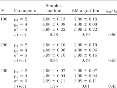
N Parameters method EM algorithm tEM/tSim
N Parameters method EM algorithm tEM/tSim
100 1⫽2 2.00⫾0.13 2.00⫾0.13 100 a1⫽25 25.00⫾0.16 25.01⫾0.16
a2⫽30 30.00⫾0.11 30.00⫾0.11
2⫽4 4.00⫾0.08 4.00⫾0.08
2⫽6 5.99⫾0.22 5.99⫾0.22 b
1⫽10 10.05⫾1.01 10.04⫾1.01
b2⫽8 8.01⫾0.38 8.01⫾0.38
t(sec) 0.38 0.19 0.50
r1⫽0.9 0.90⫾0.04 0.90⫾0.04
r2⫽0.8 0.80⫾0.02 0.80⫾0.02
200 1⫽2 2.00⫾0.10 2.00⫾0.10
2⫽4 4.00⫾0.06 4.00⫾0.06 2⫽6 5.97⫾0.22 5.97⫾0.22
t(sec) 3.5 17.5 5.0
2⫽6 5.99⫾0.16 5.99⫾0.16
t(sec) 0.84 0.19 0.53
200 a1⫽25 24.99⫾0.11 24.99⫾0.11
400 1⫽2 2.00⫾0.07 2.00⫾0.07 a2⫽30 30.00⫾0.07 30.00⫾0.07
b1⫽10 10.09⫾0.71 10.08⫾0.71
2⫽4 4.00⫾0.04 4.00⫾0.04
2⫽6 5.99⫾0.11 5.99⫾0.11 b
2⫽8 8.01⫾0.27 8.01⫾0.27
r1⫽0.9 0.90⫾0.03 0.90⫾0.03
t(sec) 1.75 0.81 0.45
r2⫽0.8 0.80⫾0.01 0.80⫾0.01
2⫽6 5.98⫾0.16 5.98⫾0.16
t(sec) 7.0 35.5 5.1
quickly when the complexity of the function increases.
400 a1⫽25 25.00⫾0.08 25.00⫾0.08
Second, in practice it typically requires only one or two
a2⫽30 30.00⫾0.05 30.00⫾0.05
function evaluations to construct a new simplex in one
b1⫽10 10.03⫾0.50 10.03⫾0.50
iteration; thus it runs very fast. Third, it is easy to
imple-b2⫽8 8.01⫾0.19 8.01⫾0.19
ment with existing computer software, such as Matlab,
r1⫽0.9 0.90⫾0.02 0.90⫾0.02
which provides a user-friendly functionfminsearchfor a r
2⫽0.8 0.80⫾0.01 0.80⫾0.01
direct usage of the method. The computer source code 2 5.99⫾0.11 5.99⫾0.11
is also downloadable from the Internet. t(sec) 20.0 75.5 3.8
Because of these favorable properties of the simplex algorithm, this algorithm has been used by some au-thors to map complex traits (Martinez et al. 1998;
Y, affected by a putative QTL of genotypesQq(denoted Perez-EncisoandVarona2000;Liuet al. 2001;
Perez-by 1) andqq(denoted by 0), is formulated as Enciso et al. 2002). However, all of these studies
pre-sented only a simple utilization of the simplex algorithm
L(Y|⍀)⫽
兿
N
i⫽1
[p f1(Yi)⫹(1⫺ p)f0(Yi)], (2)
to QTL mapping with no detailed discussion on its ad-vantages in computational efficiency and mathematical
where the vector⍀⫽(m1,m0,兺)Tcontainskexpected
manipulation and its disadvantages in some asymptotic
genotypic values, m1 and m0, for each QTL genotype
properties. Some of these studies did not cite even the
and a (k ⫻ k) within-genotype residual (co)variance seminal article by Nelder and Mead(1965). Clearly,
matrix,兺. We implement the simplex algorithm to ob-with no such discussion, the broad implications of the
tain the maximum-likelihood estimates (MLE) of⍀. simplex algorithm remain unjustified. In this note, we
Simulations: Two simulation strategies are designed for the first time compare the results and computational
to compare the results from the simplex algorithm and efficiency for QTL mapping between the simplex
algo-the EM algorithm. The first strategy considers nonfunc-rithm and the standard algononfunc-rithm. We demonstrate that
tional mapping, in which k-dimensional phenotypic the simplex algorithm is an advantageous alternative
traits measured have identical means for each QTL ge-when the purpose of a genome project is to map
dy-notype group,i.e.,m1 ⫽ 1k⫻11and m0 ⫽ 1k⫻10, and a
namic QTL that govern developmental trajectories.
constant residual variance (there are no correlations As a special case of the mixture model (Equation 1),
between the m traits), i.e., 兺 ⫽ Ik⫻k2. The data are
suppose that there is a progeny population of sizeNin
simulated under a multivariate normal distribution, with which there are two different genotype groups at each
different sample sizes (100, 200, and 400). Other simula-locus with respective frequenciespand 1⫺ p. LetY⫽
tion conditions are the heritability of 0.15 for each trait, (Y1, . . . ,YN) beNindependent observations each
hav-a tothav-al ofk⫽15 phenotypic traits, and the QTL genotype ing k-dimensional phenotypic measurements. On the
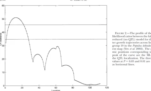
Figure2.—The profile of the log-likelihood ratios between the full and reduced (no QTL) model for diame-ter growth trajectories across linkage group 10 in thePopulus deltoides par-ent map (Yinet al.2002). The geno-mic positions corresponding to the peak of the curve are the MLEs of the QTL localization. The threshold values atP⫽0.05 and 0.01 are given as horizonal lines.
of the estimated parameters are calculated from 1000 the traditional EM algorithm. This advantage is particu-larly striking if one is using a permutation argument to simulations. All calculations are carried out on Dell
Workstation PWS530. establish significance levels, as the calculation using the
simplex algorithm would be substantially faster than the Table 1 summarizes the results from the simplest
model in which the hypothesized trait is measured only EM algorithm.
A worked example:The example for functional map-at a single time point. The MLEs of mean values and
residual variances of the trait are compared from the ping used in an outcrossing poplar byMaet al.(2002) is reanalyzed in this study. A full-sib family of 90 progeny simplex and EM algorithms. To prevent possible
occur-rences of local maxima, multiple tries for initial values was genotyped at a number of pseudo-test backcross mo-lecular markers (Yinet al. 2002). Stem diameter growth were made for the simplex algorithm. The two
algo-rithms give identical estimates of all the parameters and was measured at the end of each growing season. Ma
et al.’s (2002) functional mapping model based on the identical likelihood values for each sample size. For this
simplest situation, the simplex algorithm needs a slightly EM algorithm has successfully identified a major QTL (P⬍0.01) for 11-year diameter growth trajectories on longer computational time than the EM algorithm,
sug-gesting that the former is not advantageous for multivar- linkage group D10. This major QTL is also identified by the simplex algorithm in this study (Figure 2). As iate trait mapping.
The second simulation strategy incorporates logistic expected, the simplex and EM algorithms produce an identical profile of the log-likelihood ratios for the full growth models into the mixture-based likelihood
frame-work in Equation 2 (Maet al. 2002;Wuet al. 2002). The model (there is a QTL) vs. reduced model (there is no QTL) across the length of linkage group 10, thus expected genotypic values for each QTL genotype at
different times are modeled by m1⫽(a1/(1⫹b1e⫺r1), providing the same estimates of the two different growth
curves each for a QTL genotype. But the simplex algo-. algo-. algo-. ,a1/(1⫹b1e⫺r1k)) andm2⫽ (a2/(1⫹b2e⫺r2), . . . ,a2/
rithm uses only 85 seconds to finish a chromosome-(1⫹ b2e⫺r2k)). The results of the MLEs of growth
para-wide QTL search, whereas the EM algorithm needs 122 meters from functional mapping are almost identical
between the simplex algorithm and the EM algorithm seconds. This difference will be amplified by the number of permutation tests used to characterize the critical for all different sample sizes (Table 2). Yet, the
computa-tion times are substantially reduced when the simplex threshold for declaring the presence of QTL.
Concluding remarks: Optimization techniques, e.g., algorithm is used. On average, the time used for the
simplex algorithm is only one-fifth of that for the EM the simplex algorithm, have been used to map QTL affecting a complex trait (Martinezet al. 1998;Perez -algorithm. Thus, the simplex algorithm has a significant
and C.Cannings. Wiley, New York.
rence of global maxima. More recently, the implication
Jansen, R. C., andP. Stam, 1994 High resolution of quantitative traits
of advanced optimization techniques like genetic algo- into multiple loci via interval mapping. Genetics136:1447–1455. Knott, S. A., and C. S. Haley, 2000 Multitrait least squares for
rithms has been recognized for mapping epistatic or
quantitative trait loci detection. Genetics156:899–911.
linked QTL (Carlborget al.2000;Nakamichiet al.2001),
Lagarius, J. C., J. A. Reeds, M. H. WrightandP. E. Wright, 1998
but no attempt was made to identify their roles in func- Convergence properties of the Nelder-Mead simplex method in
low dimensions. Soc. Ind. Appl. Math. J. Optim.9:112–147.
tional mapping aimed at the identification of more
bio-Lander, E. S.,andD. Botstein, 1989 Mapping Mendelian factors
logically relevant dynamic QTL (Maet al. 2002).
underlying quantitative traits using RFLP linkage maps. Genetics
In this study, we incorporated the Nelder-Mead sim- 121:185–199.
Liu, X.-J., F. Olover, S. D. M. Brown, A. DennyandP. D. Keightley,
plex algorithm into the framework of QTL mapping.
2001 High-resolution quantitative trait locus mapping for body
Our simulation study suggests that the simplex
algo-weight in mice by recombinant progeny testing. Genet. Res.77:
rithm obtains the same results as the traditional EM al- 191–197.
Ma, C. X., G. CasellaandR. L. Wu, 2002 Functional mapping of
gorithm, but it uses different amounts of computational
quantitative trait loci underlying the character process: a
theoreti-time from the EM algorithm. If QTL mapping is
per-cal framework. Genetics161:1751–1762.
formed for a trait measured at a single point, the simplex Martinez, M., N. Vukasinovic, A. E. FreemanandR. L. Fernando,
1998 Mapping QTL in outbred populations using selected
sam-algorithm, although simple to implement, uses a longer
ples. Genet. Sel. Evol.30:453–468.
time and, hence, displays no advantage, as compared to
Nakamichi, R., Y. UkaiandH. Kishino, 2001 Detection of closely
the EM algorithm. However, for functional mapping of linked multiple quantitative trait loci using a genetic algorithm.
Genetics158:463–475.
a complex trait undergoing a particular developmental
Nelder, J. A., andR. Mead, 1965 A simplex method for function
trajectory, the simplex algorithm is much more
compu-minimization. Comput. J.7:308–313.
tationally efficient, as well demonstrated by both simula- Perez-Enciso, M., andL. Varona, 2000 Quantitative trait loci
map-ping in F2crosses between outbred lines. Genetics155:391–405.
tion and real-world examples. In conjunction with its
Perez-Enciso, M., A. Clop, J. M. Folch, A. Sanchez, M. A. Oliver derivative-free nature and easy implementation with
soft-et al., 2002 Exploring alternative models for sex-linked
quantita-ware, therefore, the simplex algorithm provides an ex- tive trait loci in outbred populations: application to an Iberian⫻
Landrace pig intercross. Genetics161:1625–1632.
cellent alternative to estimate the mixture-based model
Press, W. H., S. A.Teukolsky, W. T.Vetterlingand B. P.Flannery,
for functional mapping.
1992 Numerical Recipes in C, Ed. 2. Cambridge University Press, Cambridge/London/New York.
We thank Max Shen for his contribution of expertise to this work
Price, C. J., I. D. CoopeandD. Byatt, 2002 A convergent variant and Chris Haley for bringing to our attention the literature of the simplex
of the Nelder-Mead algorithm. J. Optim. Theor. Appl.113:5–19. algorithm for QTL mapping. This work is partially supported by grants
Sillanpaa, M. J., andE. Arjas, 1999 Bayesian mapping of multiple from the National Science Foundation to G.C. (DMS9971586) and by
quantitative trait loci from incomplete outbred offspring data. the Outstanding Young Investigator Award of the National Natural Genetics151:1605–1619.
Science Foundation of China (30128017) and the University of Florida Walters, F. H., L. R. Parker, S. L. MorganandS. N. Deming, 1991 Research Opportunity Fund (02050259) to R.W. The publication of Sequential Simplex Optimization. CRC Press, Boca Raton, FL. this article is approved as journal series R-10067 by the Florida Agricul- Wolf, J. B., 2002 The geometry of phenotypic evolution in
develop-mental hyperspace. Proc. Natl. Acad. Sci. USA99:15849–15851. tural Experiment Station.
Wu, R. L., C.-X. Ma, M. R. Chang, R. C. Littell, S. S. Wuet al., 2002 A logistic mixture model for characterizing genetic deter-minants causing differentiation in growth trajectories. Genet. Res.79:235–245.
LITERATURE CITED
Yin, T. M., X. Y. Zhang, M. R. Huang, M. X. Wang, Q. Zhugeet al.,
Carlborg, O., L. AnderssonandB. Kinghorn, 2000 The use of 2002 Molecular linkage maps of the Populus genome. Genome a genetic algorithm for simultaneous mapping of multiple inter- 45:541–555.
acting quantitative trait loci. Genetics155:2003–2010.