ABSTRACT
FAUGL, TIMOTHY ALLEN. Modeling of Visualization Cyclotron Target with Coupling of Proton Range and Target Density. (Under the direction of Dr. J. M. Doster and Dr. M. Stokely.)
©Copyright 2014 by Timothy Allen Faugl
Modeling of Visualization Cyclotron Target with Coupling of Proton Range and Target Density
by
Timothy Allen Faugl
A thesis submitted to the Graduate Faculty of North Carolina State University
in partial fulfillment of the requirements for the Degree of
Master of Science
Nuclear Engineering
Raleigh, North Carolina 2014
APPROVED BY:
Dr. R. White Dr. I. Bolotnov
Dr. J. M. Doster
Co-chair of Advisory Committee
Dr. M. Stokely
BIOGRAPHY
ACKNOWLEDGEMENTS
TABLE OF CONTENTS
LIST OF TABLES . . . vi
LIST OF FIGURES . . . vii
Chapter 1 Introduction . . . 1
1.1 Background . . . 1
1.2 Purpose . . . 3
1.2.1 Project Outline . . . 4
1.3 Related Work . . . 4
Chapter 2 Visualization Target Overview. . . 5
2.1 Design . . . 5
2.2 Experiment . . . 7
Chapter 3 Computational Model of Visualization Target . . . 8
3.1 Radiation Transport via MCNPX . . . 8
3.2 CFD Implementation via ANSYS CFX . . . 10
3.2.1 Geometry and Mesh Definition . . . 11
3.2.2 Physics, Initial Conditions, and Boundary Conditions Specification . . . . 14
3.2.3 Solver . . . 17
3.2.4 Results . . . 19
Chapter 4 Coupling of Radiation Transport to Fluid Properties . . . 24
4.1 Operating Beam Current . . . 24
4.2 Method . . . 25
4.3 Model Adaptations . . . 28
4.3.1 Computational Expense . . . 28
4.3.2 Mesh Study . . . 32
4.4 Results . . . 35
4.4.1 Full Model and Iterative Model Results Comparison . . . 36
4.4.2 Original and Iterated Beam Comparison . . . 40
4.4.3 Experimental Validation . . . 42
Chapter 5 Conclusion . . . 44
5.1 Future Work . . . 44
References. . . 46
Appendices . . . 48
Appendix A . . . 49
Appendix B . . . 51
LIST OF TABLES
Table 3.1 Domain Cell Count . . . 13
Table 3.2 Sapphire Material Properties . . . 14
Table 3.3 Domain Maximum Temperatures . . . 21
Table 4.1 Saturation Temperature Study Results . . . 24
Table 4.2 Heat Transfer Coefficient Calculation Results . . . 30
Table 4.3 Maximum Temperature Comparison: Full Model and Applied Heat Transfer Coefficient Function . . . 30
Table 4.4 Full Model and Adapted Model Comparison . . . 36
Table 4.5 Original Beam vs. Iterated Beam . . . 40
Table C.1 Rectangle Model: Maximum Temperatures . . . 56
LIST OF FIGURES
Figure 1.1 Bragg Peak . . . 3
Figure 2.1 Visualization Target: Isometric View and Section View . . . 5
Figure 2.2 Coolant Channel Orientation . . . 6
Figure 3.1 Contour and Surface Plots of Gaussian Beam Distribution . . . 9
Figure 3.2 MCNPX Energy Deposition Plot . . . 10
Figure 3.3 Original (a) and Simplified (b) Geometries . . . 11
Figure 3.4 Target Mesh . . . 12
Figure 3.5 Mesh Boundary Layer: Target Water Chamber (a) and Coolant Channel(b) . 13 Figure 3.6 Beam Distributions: MCNPX (a) and ANSYS CFX (b) . . . 20
Figure 3.7 Target Water Temperature Distribution . . . 21
Figure 3.8 Target Body Temperature Distribution . . . 22
Figure 3.9 Target Water Velocity Streamline . . . 23
Figure 4.1 MCNPX Discretization Scheme . . . 25
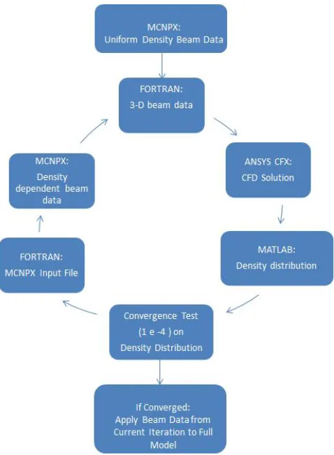
Figure 4.2 Iterative Process Flow Chart . . . 27
Figure 4.3 Coolant Channel Labeling Definition . . . 29
Figure 4.4 Target temperature profiles: Original (a) and HTC Function (b) . . . 31
Figure 4.5 Target water velocity streamlines : Original (a) and HTC Function (b) . . . . 31
Figure 4.6 First mesh change: smaller elements . . . 33
Figure 4.7 Extended Boundary Layer Mesh (a) and Beam Distribution (b) . . . 34
Figure 4.8 Adapted Mesh (a) and Beam Distribution (b) . . . 35
Figure 4.9 Density Residual Convergence Plot . . . 36
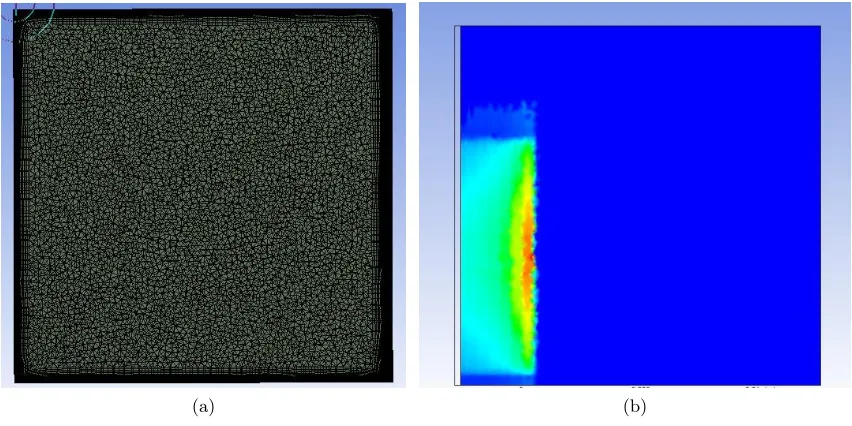
Figure 4.10 Full (a) and Iterative (b) Model Beam Distributions . . . 37
Figure 4.11 Full (a) and Iterative (b) Models Target Body Temperature Distributions . . 38
Figure 4.12 Full (a) and Iterative (b) Models Target Water Temperature Distributions . . 38
Figure 4.13 Target Water Temperature Difference (∆T) inoF . . . 39
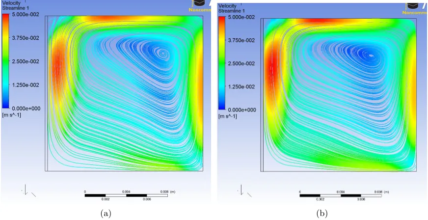
Figure 4.14 Full (a) and Iterative (b) Models Target Water Velocity Streamlines . . . 39
Figure 4.15 Original (a) and Iterated (b) Beam Distributions . . . 40
Figure 4.16 Line Plot - Original and Iterated Beam Centerline . . . 41
Figure 4.17 Original (a) and Iterated (b) Temperature Distributions . . . 42
Figure 4.18 Experimental and Computational Beams . . . 43
Figure B.1 Momentum and Mass Residual Plot . . . 52
Figure B.2 Heat Transfer Residual Plot . . . 53
Figure B.3 Turbulence (KE) Residual Plot . . . 54
Figure C.1 CAD Model: Rectangular Target . . . 55
Figure C.2 Rectangle Model: Energy Deposition Distribution . . . 56
Figure C.3 Rectangle Model: Target Temperature Distribution . . . 57
Figure C.5 Rectangle Model: Target Water Velocity Streamlines . . . 59
Figure D.1 CAD Model: Slant Target . . . 60
Figure D.2 Slanted Model: Target Temperature Distribution . . . 62
Figure D.3 Slanted Model: Target Water Temperature Distribution . . . 63
Chapter 1
Introduction
1.1
Background
Positron emission tomography (PET) is an in vivo medical imaging modalitiy that utilizes a ra-diolabeled molecule to track biochemical processes. Commonly used nuclides are11C,13N,15O, and18F.18F-deoxyglucose (FDG) is a radiolabeled sugar analog synthesized from18F. FDG is the primary radiopharmaceutical used in PET. Approximately 97% of18F decay is by positron (β+) emission. 18F is an effective imaging tool because positron annihilation produces two co-incident 511-keV annihilation photons that travel in opposite directions (180o). Coincidence detectors determine the location of the positron annihilation to track FDG as it is metaboli-cally trapped in the body. Cancer cells are characterized as being very metabolicly active, so an increased concentration of FDG is trapped in these cells. The increased positron annihilation in these areas allows an image to be constructed from the coincident detector signals.
de-sired amount of the radioisotope. This generates a significant amount of heat within the target medium, so the main focus for target design is heat removal capability.
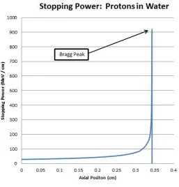
A proton deposits energy via collisions as it travels through the water. The average amount of energy lost per unit length as a charged particle travels through a medium is called the stopping power. Stopping power is most commonly used in the units MeV cm−1 and is represented by the term−dEdx [14]. The stopping power of a proton is given by the Bethe Formula for Stopping Power (Equation 1.1).
−dE
dx =
4πk02z2e4n mc2β2 [ln
2mc2β2 I(1−β2) −β
2] (1.1)
where:
k0= 8.99×10⁹ N m2C−2,
z = atomic number of the charge particle,
e= magnitude of the electron charge,
n= number of electrons per unit volume in the medium,
m = electron rest mass,
c = speed of light in vacuum,
β = Vc = speed of the particle relative to c,
I = mean excitation energy of the medium.
As the the energy of the particle approaches zero,β approaches zero. The logarithmic term decreases, causing an increase in the stopping power called the Bragg Peak [14] (shown for 18 MeV protons in water in Figure 1.1). The distance traveled per unit energy of the proton is found by taking the reciprocal of the stopping power. Using this, the range of a particle of kinetic energyT can be found using Equation 1.2:
R(T) = Z T
0
(−dE
dx)
−1dE. (1.2)
Figure 1.1: Bragg Peak
heat tranfer capabilities of various cyclotron targets using Monte Carlo Radiation Transport and Computational Fluid Dynamics (CFD) software. All previous modeling for boiling water targets has been done using assumptions for the distribution of void under saturation conditions [11]. To investigate void distribution, BTI Targetry developed a visualization target that would allow video recording of the target chamber during irradiation. The target was sufficiently robust to operate under conditions that are consistent with typical18F production targets.
1.2
Purpose
the medium. As the target water is heated by the energy deposition from the proton beam, a non-uniform density distribution develops within the target water. As the location of highest temperature should be located at the Bragg peak of the proton beam, it is expected that the fluctuation of the density at this point will affect the range of protons. This effect on the range will be magnified when the target water transitions from single phase liquid to boiling. The scope of this project is to couple the energy deposition profiles computed with the MCNPX radiation transport code with the fluid density distribution from ANSYS CFX for a target with single phase liquid. The beam current was kept at a level that did not result in temperatures exceeding the saturation temperature at the operating pressure.
1.2.1 Project Outline
First, an initial computational model was developed to provide a solution that offered acceptable agreement with the experiemental results. This inital model and corresponding results are discussed in Chapter 3. After the analysis of these results, several adaptations were made to the initial model to improve resolution and computational expense that would allow for this model to be used as an iterative step within an algorithm that couples the beam data to the fluid results. These adaptations to the initial model and the results from the iterative method are presented in Chapter 4.
1.3
Related Work
Chapter 2
Visualization Target Overview
In this section, the design of the visualization target is examined. All design work and experi-mentation was completed by BTI Targetry, LLC.
2.1
Design
(a) (b)
The visualization target water chamber was designed to have a similar volume to a typical production target chamber. The target water chamber dimensions are 14×15 ×15 mm (max fill volume of 3.15 mL). The 0.005 inch beam window is integrated into the target body and there are two viewing windows.
The visualization target must operate at the same range of particle energies and beam currents as current producation targets. This required material choices with similar thermal properties and a cooling system capable of removing the heat deposited by the proton beam. The target body is made of Aluminum 6061-T because it is a low cost, machinable metal with thermal conductivity that allows for adequate heat transfer. For the viewing windows, optically clear sapphire (Al2O3) was chosen for its ability to withstand the operating pressures as well as significantly higher thermal conductivity when compared to standard glass. The cooling system uses liquid water pumped through a system of cooling channels through the target body. The
Figure 2.2: Coolant Channel Orientation
the target body. Figure 2.2 is an image of the coolant channel orientation as described above. There are three extensions from the coolant channels into the target body that were necessary because of the machining techniques used to fabricate the target. These channels extensions are closed by flanges and are not active flow channel inlets or outlets.
2.2
Experiment
Chapter 3
Computational Model of
Visualization Target
A computational model was developed for the visualization target. This model was developed as a simple, initial solution to be compared against the experimental results to validate the effectiveness of MCNPX beam data applied as a heat source within a CFD model.
3.1
Radiation Transport via MCNPX
MCNPX is a Monte Carlo radiation transport code provided by the Department of Energy that models particle interation. This program was used to create energy deposition data tallies from proton interaction with the target water and the aluminum beam window. MCNPX generates this data from an input file that defines the domains, materials, material properties, particle type, particle energy, and beam radius [2].
fx = 2
√
2 ln 2σx (3.1)
fy = 2
√
2 ln 2σy (3.2)
The beam was modeled with a 50% transmission for 18 MeV protons. The FWHM for the desired transmission percentage and beam radius was calculated with a MATLAB code that integrated over the Gaussian distribution function with increasing σx and σy until the trans-mission percentage reached the desired amount (50%). This integration is shown in Equation 3.3. 2π Z 0 5 Z 0 1 2πσxσy
e−(
(rcosθ)2 2σx2 +
(rsinθ)2
2σ2y )rdrdθ (3.3)
σx and σy were found to be 4.2410 mm for 50% transmission, yielding a FWHM of 9.9868 mm for both the x and y directions. A two and three-dimensional plot of the Gaussian beam distribution is shown in Figure 3.1. A representative plot of the proton energy deposition tally
is shown in Figure 3.2. The scale is relative to energy deposition.
Figure 3.2: MCNPX Energy Deposition Plot
A target geometry is created within an MCNPX model via specified planes that serve as boundaries. Each domain space is identified by the plane boundaries that surround it. The material definition for that cell is specified by the chemical formula for the material and user specified density. For this beam model, the beam window and target water were specified as cylinders since the beam collimator projects the beam in a cylindrical shape through the beam window and target water. For the initial calculations, a uniform density was applied to the water domain for the energy deposition calculations.
3.2
CFD Implementation via ANSYS CFX
ANSYS CFX is a CFD software package capable of modeling fluid flow and heat transfer for solid and fluid domains. It includes four software modules that pass information required for the model analysis. The modeling process has four basic phases:
2. Physics, Initial Conditions, and Boundary Conditions Specification
3. Solver
4. Post-Processing the Results from the Solver
3.2.1 Geometry and Mesh Definition Geometry
(a) (b)
Figure 3.3: Original (a) and Simplified (b) Geometries
versions of the CAD model used in this study (view of the simplified geometry magnified).
Mesh Definition
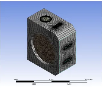
Figure 3.4: Target Mesh
(a) (b)
Figure 3.5: Mesh Boundary Layer: Target Water Chamber (a) and Coolant Channel(b)
Table 3.1: Domain Cell Count
Domain Cell Total
Target 1,384,171
Target Water 33,710
Coolant 3,149,234
Sapphire Windows 14,776
number of cells within each computational domain.
y+= u∗·y
v (3.4)
where
u∗ =
rτ w
ρ (3.5)
A y+ <11 places the first element within the viscous sub-layer region of the fluid [9]. This is critical for proper resolution in areas where the near wall velocities and temperatures are being analyzed. The mesh for the target water chamber was meshed with a maximum y+ value of approximately 3, allowing full resolution of the wall boundaries. The mesh scheme for the target water chamber and the coolant channel for this phase of the study is shown in Figure 3.5.
3.2.2 Physics, Initial Conditions, and Boundary Conditions Specification Material Specifications
The target body material specification was for the default aluminum values provided in the ANSYS CFX material libraries. Both the coolant and target water were specified as liquid water, with fluid properties provided from a table as a function of current temperature and pressure. Sapphire was not provided within the material library, so a material was defined. The properties required for the material specifictation and their respective values are provided in Table 3.2 [5].
Table 3.2: Sapphire Material Properties
Chemical Formula Al2O3
Density 3.98 g cm−1
Initial and Boundary Conditions
The initial temperature specification of the solid domains is 60o F. The exterior boundaries of the target are set to adiabatic for heat transfer. The exterior boundaries of the physical target are within the vacuum chamber of the cyclotron, so only radiative heat transfer is physically valid. The amount of heat transfered from the target via this method is neglible compared to the heat removed from the target via the coolant, so an adiabatic specification for these boundaries is within an acceptible amount of error. The boundary condition between the fluid domains and the solid domains are set as a no slip wall condition. This gives a zero fluid velocity at the wall boundary. The heat transfer mechanism between the fluid and solid domains is conjugate heat transfer with no contact resistance. This allows for calculation of heat flux via the convective heat transfer mechanism. The boundaries between the sapphire windows and the aluminum target body are set as a domain interface with calculation of heat transfer via conduction between the two materials. A contact resistance of 900 W m−2 K−1 was applied to the domain interfaces between the sapphire and aluminum domains [13].
Turbulence Model
While the Navier-Stokes equations are theoretically capable of solving the laminar and turbulent flow regions, the computational expense necessary to resolve these regions is so high that current computational capabilities are inadequate [1]. Instead, various turbulence models have been created to resolve the effects of turbulence on fluid flow. The most popular turbulence models are characterized as two-equation models. ANSYS CFX only allows for one turbulence model to be used within a single computational model, so a turbulence model that was capable of solving for the fluid flow within the target water chamber and the coolant channels was necessary.
The standard k-model was chosen for this study [8]. It is an accurate, robust model that is applicable for the majority of flow situations. The k-model introduces two new variables: k and [1]. These variables come from the differential transport equations for turbulence kinetic energy and turbulence dissipation rate, given in Equation 3.6 and 3.7, where k is the turbulent kinetic energy with units m2 s−2 and is the eddy dissipation with units m2 s −3.
δ(ρk)
δt + δ δxj
(ρUjk) =
δ δxj
[(µ+ µt
σk )δk
δxj
] +Pk−ρ+Pkb (3.6)
δ(ρ)
δt + δ δxj
(ρUj) =
δ δxj
[(µ+µt
σ ) δ
δxj ] +
k(C1Pk−C2ρ+C1Pb) (3.7)
C1, C2, σk,andσ are constants, Pkb and Pb are the buoyancy force influences, and Pk is the turbulence production from viscous forces. This model is used to solve for the turbulent viscosity, given by Equation 3.8.
µt=Cµρ
k2
(3.8)
of the boundary layer are important. Properly resolving the boundary layers within the coolant channels proved to be computationally very expensive, as the channels have physically small diameters (1 mm). For this reason, the mesh chosen for the coolant channels was allowed to have a y+ > 30. The boundary layer definition within the coolant channels (shown in Figure 3.5) was sufficient to provide a convergent solution, and kept computational costs down.
Proton Beam Data
The proton beam data is input into ANSYS CFX using a three-dimensional interpolation func-tion. MCNPX outputs a tally sheet with heat generation rates over a specified set of cells expressed in cyclindrical coordinates. A FORTRAN code was written to translate the tally output from MCNPX for a specified beam current into a three-dimensional pointwise heat gen-eration table in Cartesian coordinates. These points can be imported into ANSYS CFX, which then calculates an interpolation function that is applied to the beam window and target water. This interpolation function is included in the solution stage as an energy source. This inter-polation function can be view in the post-processor as a distribution by specifying a variable within the set-up that tracks the nodal values of the interpolation function.
3.2.3 Solver
CFD software packages solve the Navier-Stokes equations to model heat transfer, fluid flow, and other physical processes for specified domains and boundary conditions. ANSYS CFX uses the Finite Element Method (FEM) to solve the unsteady Navier-Stokes equations in conservative form. The non-linear equations are linearized and are then solved by an Algebraic Multigrid solver[4]. The instantaneous mass, momentum, and energy conservation equations are given by Equations 3.9-3.15 [1]:
δρ
δ(ρU)
δt +∇·(ρU
O
U) =−∇p+∇·(µ(∇U+ (∇UT −2
3δ∇·U))) +SM (3.10)
δ(ρhtot)
δt −
δp
δt +∇·(ρUhtot) =∇·(λ∇T) +∇·(U·τ) +U·SM +SE (3.11)
where∇·(U·τ) is the viscous work term,U·SM is the external momentum source work term, and SE is the external energy source term. The total enthalphy (htot) is related to the static enthalpy (h(T, P)) by Equation 3.12:
htot=h+ 1 2U
2 (3.12)
Applying the k-model gives the new set of Navier-Stokes equations:
δρ δt +
δ δxj
(ρUj) = 0 (3.13)
δρUi
δt + δ δxj
(ρUiUj) =−
δp0 δxi
+ δ
δxj [µef f(
δUi
δxj +δUj
δxi
)] +SM (3.14)
δ(ρhtot)
δt −
δp
δt +∇·(ρUhtot) =∇·(λ∇T+ µt
P rt
∇h) +∇·(U·τ) +U·SM +SE (3.15)
where µef f is the effective viscosity given by Equation 3.16 (µt defined in Equation 3.8), and p0 is the modified pressure given by Equation 3.17.
p0 =p+2 3ρk+
2 3µef f
δUk
δxk
(3.17)
The above equations have no general analytic solution, requiring a iterative numerical so-lution. The equations are discretized and solved numerically using FEM to calculate the mass, momentum, energy, and turbulence variables. These solutions are iterated upon until a user selected convergence criteria has been met. The default value for convergence is set for a rela-tive L2 norm, Root Mean Squared (RMS), residual (Equation 3.18) at 1 e -4 in ANSYS CFX. This value is used as the primary residual value goal used in this study. An example residual convergence plot is given in the Appendix.
kxk2= ( n X
i=1
|xi|2)
1
2 (3.18)
3.2.4 Results
The computational model for the visualization target with a 10µA beam of 18 MeV protons (180 W total energy input) with the settings described above was run with 8 partitions on 8 Intel Xeon Processors computational cores on the Henry 2 cluster. It took approximately 72 hours to reach the default convergence criteria 1e-4.
Proton Beam Energy Deposition
(a) (b)
Figure 3.6: Beam Distributions: MCNPX (a) and ANSYS CFX (b)
could be achieved by reducing the mesh element size within ANSYS CFX. However, this would increase the computational costs of the model. At this phase of the study, a precise resolution and location of the Bragg peak was not critical, so this mesh was sufficient. However, the mesh was refined for later phases of the study.
Temperature
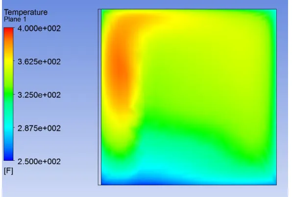
The maximum temperature computed within the model is found just above the top of the Bragg peak in the target water, shown in Figure 3.7. The maximum temperature in the target body is located at the center of the beam strike in the target window. The maximum temperatures for each domain is listed in Table 3.3.
Figure 3.7: Target Water Temperature Distribution
Table 3.3: Domain Maximum Temperatures
Domain Temperature (o F)
Target Water 387.58
Target 141.48
Sapphire Windows 334.77
Coolant 63.27
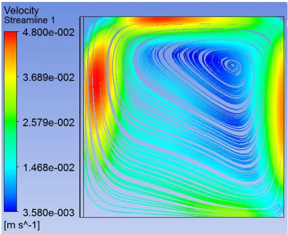
Velocity
Figure 3.8: Target Body Temperature Distribution
Chapter 4
Coupling of Radiation Transport to
Fluid Properties
4.1
Operating Beam Current
The first step in coupling the beam data to the fluid properties was to select an operating beam current. The beam current selection required a large enough margin between the maximum fluid temperature in the target water domain and the saturation temperature at the operating pressure.
Table 4.1: Saturation Temperature Study Results
Beam Current (µA) Maximum Temperature (oF)
10 387.581
13 427.369
14 441.147
15 457.141
This is critical because ANSYS CFX does not model the transition from single phase liquid into boiling. Any temperatures above the saturation temperature would result in the model no longer being physically valid.
Using the computational model, a study was done to find the minimum beam current at the selected operating conditions that results in temperatures above the saturation temperature. The results are shown in Table 4.1. The model ceases to be valid between 14 µA and 15 µA. Rather than operate at the highest possible beam current, 10 µA was chosen as the operating temperature to reduce the risk of the new beam data causing the fluid temperatures to exceed the saturation temperature. Experimental results confirm that boiling does not occur at 10µA for the visualization target operated at 300 psi, giving confidence that this is an appropriate choice for a beam current selection.
4.2
Method
Figure 4.1: MCNPX Discretization Scheme
applied from the CFD results. While there is an energy deposition mesh tool within MCNPX, it does not discretize the material so there is no way to apply a different material definition within each of the deposition cells. To discretize the model, a series of planes were specified and labeled within the MCNPX input card. The target water domain was discretized radially with 5 planes, axially with 100 planes, and angularly with 12 planes resulting in 6000 individual cells within the target water domain (shown in Figure 4.1.
Each discretization cell was created by referencing the planes that formed the boundaries, and required a line within the input file specifying the cell boundaries and material definition. A FORTRAN code was written to automatically write the input text file for MCNPX. This method allowed for a different density to be applied to each individual cell, but maintain the other material properties.
Applying the density distribution from the CFD results required exporting the results from ANSYS CFX. The export format for the density distribution gave a three-dimensional point-wise density distribution. The three-dimensional points are the coordinates of the nodes of the mesh elements within ANSYS CFX. These coordinates do not coincide with the centroids of the cells within the new MNCPX discretization. To interpolate the density distribution from the CFD results, the built-in three-dimensional interpolation tool griddata3 within MATLAB was used to produce an interpolation function from the point-wise density distribution. This interpolation function was applied to the three-dimensional coordinates of the centroids of the MCNPX discretization to find the centroid density for each cell. These densities are applied to each cell via the FORTRAN code.
4.3
Model Adaptations
For the iterative method describe to be successful, several changes had to be made to the original model. These included reducing the computational expense of the model and changing the mesh for better resolution in the beam area.
4.3.1 Computational Expense
Another issue with the iterative process is the amount of computational time required for a converged CFD solution of the model. The solution to the fluid flow through the coolant channels was the largest factor in the computational expense of the model. Various methods were investigated to decouple the solution to the fluid flow through the coolant channels.
Calculated Heat Transfer Coefficient
The first method of decoupling the coolant solution from the rest of the model was to remove the fluid domain from the model and apply a calculated heat transfer coefficient as a heat flux boundary condition. The Dittus-Boelter Correlation for flow in a smooth channel when the fluid is being heated was used for this calculation, and is given by Equation 4.1,
hc=
k
d·0.023·Re
0.8·P r0.4 (4.1)
where hc is the heat transfer coefficient, k is the thermal conductivity of the water, d is the diameter of the channel,Reis the Reynolds number, andP r is the Prandtl number. The CFD solution data for the coolant fluid flow was used to find the mass flow rate through each of the channels. This mass flow rate was used in the calculation of each of the coolant channels. The coolant channels were numbered from 1 to 6, with channel 1 being the left-most channel is facing into the beam (see Figure 4.3).
Figure 4.3: Coolant Channel Labeling Definition
boundaries with an ambient coolant temperature set to 61 oF. This method reduced the time for an ANSYS run from 72 hours partitioned on 8 parallel cores to 5 hours on a 4 core machine run serially. However, the maximum temperatures within the target water were well above the saturation temperature. Applying an average calculated heat transfer coefficient to the entire channel was not successful in maintaining the desired agreement with the full model results, so a more accurate method had to be developed.
Heat Transfer Coefficient Interpolation Function
Table 4.2: Heat Transfer Coefficient Calculation Results
Channel Mass Flux (×106) Re hc
(lb hr−1ft−2) Btu ft−2 hr−1 oF−1
1 6.96328 10030 7323.26
2 6.99125 10070 7346.78
3 7.03774 10137 7385.85
4 6.98419 10060 7340.85
5 6.95650 10020 7317.56
6 6.98226 10058 7339.56
Table 4.3: Maximum Temperature Comparison: Full Model and Applied Heat Transfer Coef-ficient Function
Full Model Applied Function Model % Difference
Max. Temp. Target Water (oF) 387.185 346.798 10.43
Max. Temp. Target Body (oF) 141.48 133.802 5.43
Max. Velocity (m s−1) 5.4 5.3 1.85
(a) (b)
Figure 4.4: Target temperature profiles: Original (a) and HTC Function (b)
(a) (b)
Figure 4.5: Target water velocity streamlines : Original (a) and HTC Function (b)
MCNPX Beam Data
number of particles provides better accuracy, but also increases the amount of time to model the beam. The particle history count was lowered to 500,000 particle histories. This beam data was used until the density residual was close to the convergence criteria. The beam was then modeled with 2,000,000 particle histories. The new beam provided better beam statistics that allowed the density and beam distribution to reach the selected convergence criteria, and required less iterations to converge since the density distribution was close to the convergence criteria from the iterations with the less expensive beam.
4.3.2 Mesh Study
It was expected that the change in the beam shape would be small after the first few iterations, so a mesh that provided better resolution over the beam strike area was critical to the success of the iterative process.
Decreasing Element Size
The first change that was made to the mesh scheme was to simply reduce the size of the elements in the target water. This new mesh scheme and the resulting beam distribution is shown in Figure 4.6. While this change did effectively increase the beam resolution in the beam strike area, it also significantly increased the computational expense (from 5 hour run on 4 core machine to 36 hour run partitioned over 8 cores). This method did not meet the requirements of low computational expense and good resolution, so a new approach had to be taken.
Structured Mesh
(a) (b)
Figure 4.6: First mesh change: smaller elements
Extended Boundary Layer
(a) (b)
Figure 4.7: Extended Boundary Layer Mesh (a) and Beam Distribution (b)
Extended Boundary Layer with Bottom Layer Removed
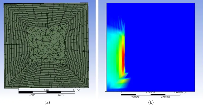
(a) (b)
Figure 4.8: Adapted Mesh (a) and Beam Distribution (b)
4.4
Results
The beam and density distribution successfully reached the convergence criteria (1e-4 maximum relative L-2 residual). Once the residual began to decrease very slowly but had not reached the convergence criteria, the number of particle histories in the MCNPX beam model was increased. This change in the beam definition caused a spike in the residual plot (see Figure 4.9). The beam data from the final iteration was then applied to the full target model, and the results were compared to the iterative model to confirm the iterative and full modeling methods had an acceptable level of agreement. The full model results with the new beam data were also compared to the original model results, as well as the experimental results.
Figure 4.9: Density Residual Convergence Plot
4.4.1 Full Model and Iterative Model Results Comparison
Table 4.4: Full Model and Adapted Model Comparison
Full Model Adapted Model % Difference
Max. Temp: Target Body (oF) 143.3534 142.1402 0.846
Max. Temp: Sapphire (oF) 338.2196 332.0240 1.832
Max. Temp: Target Water (oF) 389.8688 383.3384 1.675
Max. Velocity: Target Water (m s−1) 0.058563 0.0575216 1.778
are shown for each model in Figure 4.10. The beam data from the two models are identical, so the maximum volumetric heat generation rate is the same for both models. The temperature distributions in the target and target water (Figures 4.11 and 4.12) show excellent agreement, with maximum temperatures in the same location and less than 2% difference. A temperature difference profile for the target water between the Full model and the Iterative model is shown in Figure 4.13. The velocity differences between the two models also show less than 2% difference. There is excellent agreement between the full model and the adapted model, so the methods used to decrease the computational expense were successful and gave results with an acceptable level of agreement between the two models.
(a) (b)
(a) (b)
Figure 4.11: Full (a) and Iterative (b) Models Target Body Temperature Distributions
(a) (b)
Figure 4.13: Target Water Temperature Difference (∆T) in oF
(a) (b)
4.4.2 Original and Iterated Beam Comparison
To study the effect of coupling the beam data with the density distribution of the target water, the iterated beam data was compared to the original beam data (uniform density distribution).
Table 4.5: Original Beam vs. Iterated Beam
Original Iterated
Beam Range (mm) 3.10 4.05
Max. Q”’ (W m−3) 1.72793×10⁹ 1.38028×10⁹
Max. Temperature (o F) 362.77 383.34
(a) (b)
Figure 4.15: Original (a) and Iterated (b) Beam Distributions
than the density independent beam. The maximum volumetric heat generation rate is greater in the original beam. The density dependent beam has a broader Bragg Peak region, giving less intense area of maximum heat generation. A line plot of the volumetric heat generation rate through the center of the beam is shown in Figure 4.16. Though the maximum value of the energy deposition was lower, the iterated beam model had a higher maximum temperature.
(a) (b)
Figure 4.17: Original (a) and Iterated (b) Temperature Distributions
4.4.3 Experimental Validation
(a) (b)
Chapter 5
Conclusion
The computational model successfully coupled the MCNPX beam data with the fluid property distribution from ANSYS CFX. Applying the density distribution to the MCNPX model defi-nition increased the proton beam range by 0.95 mm (30.65%), and also resulted in a broad, less intense Bragg peak. The proton beam range and velocity profiles between experimental and computational results offer good agreement, giving confidence that this technique can be used to model the thermal performance of other target geometries.
5.1
Future Work
The next phase of this model is to apply the Homogenous Equilibrium Model (HEM) as a method of modeling the transition from single phase liquid to boiling. The HEM method assumes that the fluid and vapor phases have equal velocities and are in thermodynamic equilibrium. This can be achieved by modifying the state equations within ANSYS CFX.
deposition and beam shape is expected to be coupled much tighter to the density distribution for these targets because vapor density fluctuates much more with changes in temperature than liquid.
REFERENCES
[1] ANSYS CFX 14.0 Manual.
[2] MCNPXT M USER’S MANUAL.
[3] Iba cyclone, 2013.
[4] FEATFLOW. High performance finite elements: Used cfd software packages.
[5] MolTech Gmbh. Sapphire al2o3, 2013.
[6] Sven-Johan Heselius, Peter Lindblom, and Olof Solin. Optical studies of the influence of an intense ion beam on high-pressure gas targets. The International Journal of Applied Radiation and Isotopes, 33(8):653 – 659, 1982.
[7] Bong Hwan Hong, Tea Gun Yang, In Su Jung, Yeun Soo Park, and Hyung Hee Cho. Visu-alization experiment of 30 mev proton beam irradiated water target. Nuclear Instruments and Methods in Physics Research Section A: Accelerators, Spectrometers, Detectors and
Associated Equipment, 655(1):103 – 107, 2011. Proceedings of the 25th World Conference of the International Nuclear Target Development Society.
[8] B.E. Launder and D.B. Spalding. The numerical computation of turbulent flows. Computer Methods in Applied Mechanics and Engineering, 3(2):269 – 289, 1974.
[9] M. Nallasamy. Turbulence models and their applications to the prediction of internal flows: A review. Computers and Fluids, 15(2):151 – 194, 1987.
[11] Johanna L. Peeples, Matthew H. Stokely, and J. Michael Doster. Thermal performance of batch boiling water targets for 18f production.Applied Radiation and Isotopes, 69(10):1349 – 1354, 2011.
[12] M.E. Phelps. PET Molecular Imaging and its Biological Applications. Springer-Verlag, 2004.
[13] S. Sahling, J. Engert, A. Gladun, and R. Knoner. The thermal boundary resistance between sapphire and aluminum monocrystals at low temperature. Journal of Low Temperature Physics, 45(5-6):457–469, 1981.
Appendix A
MCNPX Input File Example
18 MeV P r o t o n s in W a t e r c M e s h E n e r g y D e p o s i t i o n c
c
c c e l l c a r d s -c
c
c A l u m i n u m
1 1 -2.810 -1 2 -3 imp : h =1 c W A T E R
2 2 -1 -1 3 -4 imp : h =1 c O U T S I D E U N I V E R S E
3 0 1: -2:4 imp : h =0
c s u r f a c e c a r d s -c
1 cz 0.5 2 pz 0.0 3 pz 0 . 0 1 2 7 4 pz 1.0
c m a t e r i a l c a r d s -c
c M a t e r i a l #1: A l u m i n u m m1 1 3 0 2 7 -1
c M a t e r i a l #2: H20
m2 H L I B =24 h 1 0 0 1 . 2 4 h -0.1119 8 0 1 6 . 2 4 h -0.8881 c d a t a c a r d s
-m o d e h
p h y s : h 1 8 . 0 j 0. j cut : h 0 . 0 5
keV min lca j j j nps 1 0 0 0 0 0 F1 : H 2
c the n e x t 7 l i n e s are the e n e r g y d e p o s i t i o n m e s h T M E S H
C M E S H 3 t o t a l E R G S H 3 0.0 1 8 . 0
C O R A 3 0.0 0 . 0 1 3 1 5 7 8 9 5 6 5 5 17 i 0 . 4 8 6 8 4 2 1 0 4 3 4 5 0.5 C O R B 3 0.0 0 . 0 2 3 6 8 4 2 1 1 2 0 4 17 i 0 . 8 7 6 3 1 5 7 8 8 7 9 6 0.9 C O R C 3 360
E N D M D c
c s o u r c e d e f i n i t i o n -c 18 MeV P r o t o n B e a m
S D E F SUR =2 DIR =1 vec =0. 0. 1. erg = 1 8 . PAR = h pos =0. 0. 0. x = d5 y = d3 z =0 CCC =1
SC3 G a u s s i a n D i s t r i b u t i o n w i t h 50% at 5.0 mm SP3 -41 0 . 9 9 8 6 8 0
Appendix B
Appendix C
Rectangle Visualization Geometry
Figure C.1: CAD Model: Rectangular Target
larger beam diameter (12 mm), which should results in a lower maximum temperature at the Bragg peak for the same particle energy and beam currents. Preliminary modeling has been performed on this geometry (initial mesh setup, uniform density beam data, and full coolant solution).
Table C.1: Rectangle Model: Maximum Temperatures
Domain Maximum TemperatureoF
Target 138.48
Sapphire 263.20
Target Water 305.82
Coolant 62.15
Figure C.3: Rectangle Model: Target Temperature Distribution
From the initial model results, the new target geometry has successfully increased the ther-mal capacity of the target system. The maximum temperatures in the target and target water are lower in the Rectangle visualization target than the original visualization target, and are located in the same corresponding areas as in the original model (Figures C.3 and D.3). The convection currents within the target water are also very clearly shown in Figure D.4.
Figure C.4: Rectangle Model: Target Water Temperature Distribution
Table C.2: Rectangle Model: Saturation Temperature Study Results
Beam Current (µA) Maximum Temperature (oF)
10 305.823
15 360.967
20 407.268
25 447.444
Appendix D
Slanted Visualization Geometry
Figure D.1: CAD Model: Slant Target
geometry. A slanted back wall was added to remove a portion of the target water chamber without affecting the natural circulation currents within the target chamber. This model has proven to be computationally very expensive. The amount of time necessary to reach the default convergence criteria exceeds 240 hours when partitioned 8 times on 8 cores. Decreasing the computational expense of this model will be a priority before future work can be completed.
The results shown below do not provide an accurate comparison to the results for the Rectangle model given in Appendix C because this model was run without a contact resistance specified between the sapphire windows and target body. This model was run prior to the value of contact resistance being provided. Though it is not appropriate to compare these results to the results in Appendix C, the results will provide insight into the temperature distribution and velocity profile.