Compositional Data Analysis and Zeros in Micro Data

Full text

(1)CENTREof POLICY STUDIESand the IMPACT PROJECT. Menzies Building Monash University Wellington Road CLAYTON Vic 3168 AUSTRALIA Telephone: (03) 990 52398, (03) 990 55112. from overseas: 61 3 990 52398 or 61 3 990 55112. Fax numbers: (03) 990 52426, (03)990 55486 e-mail. from overseas: 61 3 990 52426 or 61 3 990 55486 [email protected]. COMPO SITI ONAL DATA ANALYSIS AND. Z ERO S I N M I C RO D AT A by. Jane M. FRY Centre of Policy Studies, Monash University. Tim R.L. FRY and Keith R. MCLAREN Department of Econometrics, Monash University. General Paper No. G-120 March 1996 ISSN 1 031 9034. ISBN 0 7326 0736 1. The Centre of Policy Studies (COPS) is a research centre at Monash University devoted to quantitative analysis of issues relevant to Australian economic policy. The Impact Project is a cooperative venture between the Australian Federal Government and Monash University, La Trobe University, and the Australian National University. COPS and Impact currently operate as a single unit at Monash University with the task of constructing a new economy-wide policy model to be known as MONASH . This initiative is supported by the Industry Commission on behalf of the Commonwealth Government, and by several other sponsors. The views expressed herein do not necessarily represent those of any sponsor or government..

(2) ABSTRACT. The application of compositional data analysis methods in economics has some attraction. In particular, this methodology ensures that the stochastic component of budget share models will satisfy the restriction of shares to the unit simplex. The methodology relies upon the use of \log-ratios" in the statistical analysis. Such an approach is not possible when the data to be analyzed includes observations where the observed budget share is zero. We, therefore, extend the methods of compositional data analysis to the situation where the data to be analyzed includes observations where the observed budget share is zero. The modi¯ed compositional data methods are discussed both in statistical terms and through potential economic interpretations of the method. Further, the modi¯ed methodology is applied to the 1988 Australian Household Expenditure Survey yielding estimates for a system of Engel curves.. JEL Classi¯cation:. C51, D12. Engel Curves, Modi¯ed Almost Ideal Demand System, Compositional Data Analysis, Australian H.E.S. data. Keywords:.

(3) TABLE OF CONTENTS. 1 2 3 4 5. Introduction Compositional Data Analysis and Zeros Empirical Application Conclusions References. 1 2 3 4 5 6. List of Tables Zero Replacement Procedures Zeros in Australian Micro Consumption Data Number of Zeros MAIDS Engel Curve Estimation Results Total Expenditure Thresholds Estimated Expenditure Elasticities. Page 1 2 5 12 13 4 6 7 8, 9 10 11.

(4) COMPOSITIONAL DATA ANALYSIS AND ZEROS IN MICRO DATA Jane M. Fry ¤. Tim R.L. Fry and Keith R. McLaren. 1.. Introduction.. The statistical literature has advocated the use of compositional data analysis methods when working with data on (budget) shares (for a comprehensive review of these methods see Aitchison (1986)). This methodology has the advantage that it ensures that the stochastic component of a model for budget shares will satisfy the restriction that shares should be constrained to the unit simplex. In earlier work (Fry et al (1996), McLaren et al (1995)) we have argued that compositional data methods should be used in the econometric speci¯cation of models of budget shares. Suitably modi¯ed to allow the mean to be parameterized on the basis of economic theory, the application of this methodology yields the following estimable form for our system of equations = log. ³ i´ w. w. = log. ³ i´. ¡. W + vi ; i = 1; : : : ; N 1(= n) (1.1) WN N with w denoting the observed share, W denoting the \deterministic" component derived from economic theory and = (v1:::vn ) a multivariate normal disturbance term. This is simply a non-linear multivariate regression model and can be easily estimated with existing software for moderately large n.. yi. v. 0. If W is derived from an indirect utility function that satis¯es certain \regularity" conditions, the attraction of this approach is that the shares are bounded to the unit simplex in terms of both the deterministic and the stochastic components. Unfortunately, a problem arises if any w is zero. Traditionally in demand analysis this is avoided by assuming that quantity demanded, qi , is always positive and/or by the use of aggregate time series data. However, in microeconomic data, as collected in either expenditure surveys or in panel studies, the occurence of zero observations for shares is common. These zeros would seem to preclude the use of compositional data methods with such microeconomic data. On the other hand, the model in (1.1) does have a certain intuitive appeal in the case of zero shares. If, for a certain range of values of the exogenous variables, there is a preponderance of zero observations for the share of a particular commodity, then it ¤. This research was supported by an Australian Research Council grant. We are grateful to Alan Powell and Maureen Rimmer for helpful comments on the work reported in this paper. The usual disclaimer, however, applies.. 1.

(5) COMPOSITIONAL DATA ANALYSIS AND ZEROS IN MICRO DATA. 2. would be desirable for an estimation method to select values of the model parameters such that the deterministic part of the model also gave zeros (corner solutions) when evaluated at those values of the exogenous variables. With a Normal speci¯cation of for the the vi , the above model achieves this in that for any likely value for vi , a left hand side e®ectively forces a for the deterministic component on the right hand side. The question that remains is how to handle the in a numerical sense.. ¡1. ¡1. ¡1. The problem of zero shares is not unique to microeconomic data and the statistical literature does include discussion of this modeling situation. This paper reviews and extends the existing statistical methodology for modeling compositions with zero components (shares)1. The modi¯ed version of the compositional data analysis method is then applied to Australian household expenditure data to illustrate the modeling procedure. The plan of the rest of the paper is as follows. Section two discusses compositional data analysis and the presence of zeros. It looks at the rationalizations used for the occurence of zeros and the strategies proposed to modify the methodology. The discussion is concerned both with the statistical details and the \economic" interpretation of the strategies. Section three describes the application of the modi¯ed zero replacement methodology to estimate a system of Engel curves using the 1988 Australian household expenditure survey. Finally section four contains some concluding remarks. 2.. Compositional Data Analysis and Zeros.. In the statistical literature, two explanations for the occurence of zero observations are proposed. These are rounding (or trace elements) and \essential" (or true) zeros. The ¯rst of these rationalizes that the zero observation is an artefact of the measurement process. Basically, if we had a more accurate measurement instrument we would record a non-zero observation for the share. Thus the observed zero is a proxy for a very small number. The second rationalization argues that the observation should be zero as the true generating process leads to the occurence of zeros. The proposed modi¯cations to deal with zero observations can then be derived by considering the cause of the zero (see Aitchison (1986) pp 266-274). In terms of economic modeling we might argue that of these two causes the second is analogous to the situation of a corner solution and so, if we believe that our zeros are the result of corner solutions, the modi¯ed zero replacement methodology may be useful. On the other hand, the existence of zeros through measurement errors is potentially less likely in economic data. Although the \solutions" to the problem of zero observations are discussed by Aitchison (1986) according to the cause of the zero, we present them as competing techniques to deal with both types of zero and discuss the applicability in the case 1 An excellent summary of the economic literature concerning zeros can be found in Pudney (1989)..

(6) COMPOSITIONAL DATA ANALYSIS AND ZEROS IN MICRO DATA. 3. of microeconomic data. The techniques to be considered are amalgamation, zero (or trace) replacement, modi¯ed Box-Cox and conditional modeling2 . Amalgamation is the reduction of the number of components in the composition by the grouping together of certain components. That is, we decrease the number of commodities by aggregating into broader commodity groups. This is a simple approach and may have some attraction. However, if the emphasis of the modeling exercise is to study behavior at the disaggregate level then aggregation is a priori not an appropriate technique to deal with the zero observations. For much microeconometric work the emphasis is on disaggregate modeling and so we rule out the use of amalgamation. Zero (trace) replacement is a technique usually discussed in the context of zeros caused by the measurement process. It is, however, possible to use it no matter how the zeros arose. The zero replacement technique and the other compositional data techniques for dealing with zeros typically assume that the number of zeros for each observation is ¯xed at M and with the same components being zero for each observation. In economic data that is unlikely to be true. However, there is no reason why the techniques cannot be applied, observation by observation, with M varying. The zero replacement technique assumes that a composition has M zero and N M non-zero components. It is recommended that the zeros be replaced by \small" values. In particular, using arguments based upon a ternary representation of the data (Aitchison (1986) pp 266-267), it is suggested that we replace the zeros with 2 2 ¿A = ± (M + 1)(N M )=N and then reduce the non-zeros by ¿S = ±M (M + 1)=N , where ± is the maximum rounding error. Bounds for ± can then be set within this ternary framework.. ¡. ¡. In terms of its application to (economic) data there is a problem with this technique as it stands. The compositional data methodology relies upon the use of share ratios. The zero replacement procedure is not ratio preserving. In particular, the ratios for the non-zero shares are distorted by the zero replacement procedure. For example, consider the case where N = 5; M = 2 and ± = 0:027_ (see Table 1). In this case the two zeros are each replaced by 0.01 and the non-zeros are each reduced by the appropriate amount. This does not preserve the share ratios. An alternative procedure is to replace the zeros by the same number, ¿A , but to reduce each non-zero by wi ¿S . This both retains the share ratios for the non-zero components and makes an appropriate zero replacement. In the context of budget share. £. 2 It. has also been proposed to replace the shares by ranks (Bacon-Shone (1992)). This discards a large amount of information and will not be considered here..

(7) COMPOSITIONAL DATA ANALYSIS AND ZEROS IN MICRO DATA. 4. modeling this procedure has the appeal that the expenditure implicitly allocated as zero replacement is withdrawn from the non-zero commodities in an (approximately) optimal manner. That is, the amount taken from the non-zeros is proportional to the size of that non-zero value. We call this alternative zero replacement procedure modi¯ed Aitchison.. Table 1: Zero Replacement Procedures, N = 5 M = 2 ± = 0 027_ . ;. 1. 2. ;. Commodity (i ) 3. :. 4. 5. Observed. Expenditure ($) Share. wi yi. Aitchison. wi yi. Modi¯ed Aitchison. wi yi. 0 0.00. ¡1. 15 0.15 log(1:5). 0 0.00. ¡1. 75 0.75 log(7:5). 10 0.10. 0.01 0:01 log( 0:093_ ). 0.143_ 3_ log( 00::14 ) 093_. 0.01 0:01 log( 0:093_ ). 0.743_ 3_ log( 00::74 ) 093_. 0.093_. 0.01. 0.147 log(1:5). 0.01. 0.735 log(7:5). 0.098. 01 log( 00::098 ). :01 log( 00:098 ). £ £ £. A related issue is then the setting of an appropriate range for the zero replacement value ¿A (and hence for ± and ¿S ) in the modi¯ed Aitchison technique. In terms of expenditures the minimum value a zero should be replaced with is 0.01 (one cent). If we divide this by the maximum value of total expenditure in our data then we produce a sensible minimum value for our zero replacement ¿A . We can then ¯nd ± and ¿S . Analogously, if we divide 0.01 by the minimum value of total expenditure in our data we will produce a sensible maximum value for our zero replacement procedure. It is the combination of modi¯ed Aitchison and this setting of ¿A ; ± and ¿S that we recommend in the use of the zero replacement technique3 . Two points need to be considered in the use of zero replacement. Firstly the sensitivity to the replacement procedure. In this situation we need to consider different values of ¿A (equivalently ±) and see whether our parameter estimates change dramatically. This is essentially a robustness issue. If the estimates do not change dramatically then we can have some con¯dence in them. The second issue is whether our replacement observations are \outliers" in our statistical modeling. This issue can be assessed using the usual residual diagnostics. 3 Another approach is to argue that zero should be replaced by the smallest possible number and this could be found by assessing the numerical accuracy (storage) capacity of the software to be used in the modeling. This would have the disadvantage of introducing a potential dependence of results on the hardware or software used..

(8) COMPOSITIONAL DATA ANALYSIS AND ZEROS IN MICRO DATA. 5. As discussed in Fry et al (1996), in the case when Wi is zero (e.g. a corner solution) the compositional data methodology ensures that the modeled wi will also be zero. In that paper we argue that the problem of zeros and hence through the log transform is essentially a numerical one and we suggest using an appropriate replacement procedure. Such a procedure is the modi¯ed Aitchison procedure described in this paper. Thus zero replacement has this further advantage in econometric modeling.. ¡1. The third technique of dealing with zero observations is the use of the modi¯ed Box-Cox transformation. That is, in place of the log-ratio transformation we use: yi. =. (wi =wN )¸i ¸i. ¡1. ;. i. = 1; :::; n. (2.1). which can be applied so long as wN is always non-zero. A similar transformation is applied to the deterministic part of the model, the Wi . Unfortunately, in microeconomic data it is often the case that we do not have a commodity for which w will always be non-zero. A further problem with this approach is that the transformed distributions which are produced and de¯ne the likelihood function do not have any \nice" properties (e.g. normality). Thus likelihood based estimation is extremely di±cult4. The ¯nal nail in the co±n of this technique from an economist's perspective is that the technique is not \invariant" to the normalizing commodity, N . Conditional modeling attempts to separate out the zero components and model them and the non-zeros using conditioning arguments. For example, if zeros are con¯ned to the ¯rst M components, then it is possible to specify one model for the full composition with no zero (i.e.N ) components and another model for the subcomposition with N M components. If these models occur with probabilities ¼ and 1 ¼ respectively then the log-likelihood for the full model is a weighted sum of the log-likelihoods of the two models. This technique can be expanded and has some attraction in that it is similar the the \hurdle" models used in economics (see Pudney (1989)). However, the resultant modeling quickly becomes computationally di±cult and thus we do not recommend this technique.. ¡. ¡. Summarizing the above discussion, we can see that the modi¯ed Aitchison zero replacement technique is simple to implement, easy to work with and has the added attraction of having an economic rationale for its use. In the next section we, therefore, discuss its use in an empirical application. 3.. Empirical Application.. The household expenditure survey (HES), conducted by the Australian Bureau of Statistics, collects expenditure, income and other information on a representative 4 Least. squares techniques are also di±cult to use with Box-Cox procedures..

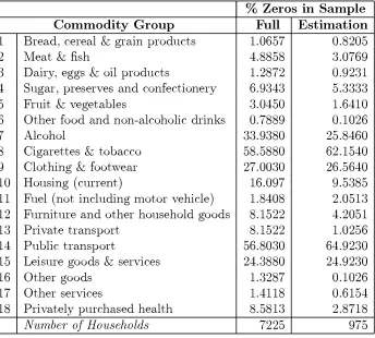
(9) COMPOSITIONAL DATA ANALYSIS AND ZEROS IN MICRO DATA. 6. sample of Australian households. The sampling methodology is broadly based upon that of the family expenditure survey (FES) in the United Kingdom and its primary use is in determining the expenditure weights for use in the consumer price index. In this study we use the 1988 HES at the household level to estimate a system of Engel curves5. The HES collects expenditure information at the \¯ne-level" of 421 commodities. We aggregate these into 18 commodity groups, comparable to those in Rimmer and Powell (1994), for use in our analysis6. Table 2 contains the percentage of zero share observations for each of our broad groups in the HES.. Table 2: Zeros in Australian Micro Consumption Data. % Zeros in Sample Commodity Group Full Estimation 1 2 3 4 5 6 7 8 9 10 11 12 13 14 15 16 17 18. Bread, cereal & grain products Meat & ¯sh Dairy, eggs & oil products Sugar, preserves and confectionery Fruit & vegetables Other food and non-alcoholic drinks Alcohol Cigarettes & tobacco Clothing & footwear Housing (current) Fuel (not including motor vehicle) Furniture and other household goods Private transport Public transport Leisure goods & services Other goods Other services Privately purchased health Number of Households. 1.0657 4.8858 1.2872 6.9343 3.0450 0.7889 33.9380 58.5880 27.0030 16.097 1.8408 8.1522 8.1522 56.8030 24.3880 1.3287 1.4118 8.5813 7225. 0.8205 3.0769 0.9231 5.3333 1.6410 0.1026 25.8460 62.1540 26.5640 9.5385 2.0513 4.2051 1.0256 64.9230 24.9230 0.1026 0.6154 2.8718 975. Source: 1988 Australian Household Expenditure Survey. We can see that no group always has non-zero share observations and the range of the problem of zero observations is large. Rather than deal with the large sample 5 The identi¯cation of relative price terms in a demand system using a cross section survey is not possible. Hence we estimate Engel curves. 6 The exact mapping of \¯ne-level" commodities to our 18 groups is available on request from the authors..

(10) COMPOSITIONAL DATA ANALYSIS AND ZEROS IN MICRO DATA. 7. size and attendant heterogeneity of the complete HES, we restrict attention to a relatively homogeneous sub-sample for our estimation. This sub-sample comprises two adult, single or dual income, no children households. The extent of the zero observation problem for this sample can also be found in Table 2. We see that although the pattern of percentages of zero shares is di®erent from the full HES, the estimation sample does contain a large zero observation problem. As such we believe that applying the modi¯ed Aitichison zero replacement technique to this data will be a good test of the usefulness of the technique. To implement the zero replacement we need to determine ¿A , ± and ¿S . Using our guidelines the minimum zero replacement value is given by 0:01=1929:85 and the maximum replacement value by 0:01=79:08. To ¯nd ± and ¿S we need to know N (=18) and M. Table 3 shows that for our data the maximum number of zeros for any observation is 8.. Table 3: Number of Zeros. Zeros (M) Count 0 1 2 3 4 5 6 7 8. 48 242 281 229 96 51 19 8 1. We therefore set M to 8 and ¯nd the values for ± and then ¿S . We ¯nd that ± min = 0:00001865 and ± max = 0:00045524. To investigate robustness to zero replacement we also consider the median value ± med = 0:00023695. The procedure is then to work through the data, observation by observation, replacing zeros with ¿A and adjusting the non-zeros by subtracting wi ¿S . This produces a \zero-replaced" data ¯le for analysis. A system of Engel curves is estimated on this \zero-replaced" data. The procedure is then repeated with di®erent values for ± and hence ¿A and ¿S . The idea is to investigate the robustness issue.. £. Regularity of the deterministic component of demand systems is important. The Almost Ideal Demand system does not always satisfy this condition and thus we choose to estimate the Modi¯ed Almost Ideal Demand system (MAIDS) of Cooper and McLaren (1992). This system is attractive since it preserves regularity over a wide region. The parameterization of MAIDS we use is to set, in the original notation,.

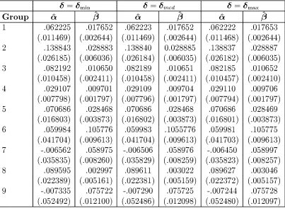
(11) COMPOSITIONAL DATA ANALYSIS AND ZEROS IN MICRO DATA. 8. P. ¯i = 1, and to normalize on minimum total income by setting K to this = value (i.e. in the original Cooper & McLaren notation: · = log(K )). This gives us regularity over all of the sample space. The MAIDS speci¯cation for the shares in our Engel curve analysis is therefore given by: ´. Wi. =. + ¯i log(Yi =K ) 1 + log(Yi =K ). ®i. (3.1). where Y is total expenditure. A further advantage of our estimation sub-sample is that we do not need to worry about the incorporation of demographic variables into the system. The results of zero replacement estimation are given in Table 4 below:. Table 4: MAIDS Engel Curve Estimation Results for Varying ±. Group 1 2 3 4 5 6 7 8 9. ®^. ± = ±min. .062225 (.011469) .138843 (.026185) .082192 (.010458) .029107 (.007798) .070686 (.016803) .059984 (.041704) -.006562 (.035835) .089595 (.022389) -.007335 (.052492). ¯^. .017652 (.002644) .028883 (.006036) .010650 (.002411) .009701 (.001797) .028468 (.003873) .105776 (.009613) .058975 (.008260) .002997 (.005161) .075722 (.012100). Table 4 continues .... ®^. ±=±. .062223 (.011469) .138840 (.026184) .082189 (.010458) .029109 (.007796) .070686 (.016802) .059983 (.041704) -.006506 (.035829) .089611 (.022381) -.007290 (.052486). med. ¯^. .017652 (.002644) 0.028885 (.006035) .010651 (.002411) .009704 (.001797) .028468 (.003873) .1055776 (.009613) .058976 (.008259) .003022 (.005159) .075725 (.012098). ®^. ± = ±max. .062222 (.011468) .138837 (.026182) .082185 (.010457) .029110 (.007794) .070686 (.016801) .059981 (.041703) -.006450 (.035823) .089627 (.022372) -.007244 (.052480). ¯^. .017653 (.002644) .028887 (.006035) .010652 (.002410) .009706 (.001797) .028469 (.003873) .105775 (.009613) .058997 (.008257) .003046 (.005157) .075728 (.012097).

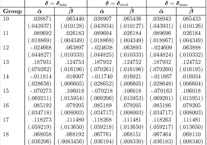
(12) COMPOSITIONAL DATA ANALYSIS AND ZEROS IN MICRO DATA. 9. Table 4 continued. Group 10 11 12 13 14 15 16 17 18. ®^. ± = ±min. .038871 (.043937) .089692 (.018869) -.024668 (.044827) .187931 (.070262) -.011814 (.028656) -.070273 (.069211) .085192 (.034718) .118273 (.059219) .068058 (.036206). ¯^. .065440 (.010128) .026183 (.004349) .063897 (.010333) .124753 (.016196) .016007 (.006605) .106018 (.015954) .079205 (.008003) .111480 (.013650) .068192 (.0083456). ®^. ±=±. .038907 (.043934) .089694 (.018868) -.024638 (.044825) .187932 (.070261) -.011740 (.028652) -.070218 (.069206) .085189 (.034717) .118268 (.059218) .067761 (.036194). med. ¯^. .065436 (.010127) .026184 (.004349) .063893 (.010333) .124752 (.016196) .016021 (.006605) .106018 (.015953) .079205 (.008003) .111481 (.013650) .068151 (.008330). ®^. ± = ±max. .038943 (.043931) .089696 (.018867) -.024609 (.044824) .187932 (.070260) -.011667 (.028648) -.070163 (.069201) .085186 (.034717) .118263 (.059217) .067464 (.036183). ¯^. .065433 (.010126) .026184 (.004349) .063888 (.010332) .124752 (.016195) .016034 (.006604) .106018 (.015951) .079205 (.008003) .111481 (.013650) .068110 (.008340). Standard errors in parentheses.. ± ±min ± ±max. med. Maximized Log-L 29680.1 29681.7 29683.3. The estimates of both the parameters and the standard errors are remarkably similar for all values of ±. In addition, interval estimates for both the ®'s and the ¯ 's based on the extreme values of ± would overlap. The parameters where the di®erences are largest are the estimates of ®18 and ¯18 . As these estimates are obtained from the adding up constraint, and so may su®er from \rounding errors" it is not surprising that they exhibit the largest di®erences. However, even these estimates are very close to each other. Thus we can have reasonable con¯dence in the robustness of the procedure. Additionally, the maximized log-likelihood values are also very close, con¯rming the robustness of the procedure. If a single set of estimates is to be used for interpretation, then perhaps those for the minimum-± replacement data should be used..

(13) COMPOSITIONAL DATA ANALYSIS AND ZEROS IN MICRO DATA. 10. Given the normalization of MAIDS achieved by setting K equal to the minimum expenditure in the sample, su±cient conditions for the regularity of the underlying demand system are that ®i ; ¯i 0; i = 1; : : : ; 18. From Table 4, with ± = ±min , all of the estimated ¯i satisfy this condition, but for ¯ve commodities (Alcohol, Clothing & footwear, Furniture and household goods, Public transport and Leisure goods & services) the estimated ®i are (insigni¯cantly) negative. One approach would be to set these ®i to zero, with the interpretation that a consumer with total expenditure equal to the minimum total expenditure would be at a corner solution for these ¯ve commodities, and would only consume positive quantities at higher levels of total expenditure.. ¸. An alternative, and more appealing interpretation, would be to maintain these point estimates as the parameter values and to write7 : ®i. + ¯i log(Yi =K ) = 0. (3.2). and solve for the implied values of Yi . For each commodity where the estimate of ®i is negative, the above equation determines that level of expenditure, Yi , at which the estimated share (and hence expenditure) for commodity i is zero. The appropriate interpretation is then that for total expenditure less than Yi expenditure on commodity i will be zero (i.e. a corner solution). For the ¯ve commodity groups with negative ®i the expenditure levels which act as the thresholds are given in Table 5. The ordering and magnitudes of these total expenditure thresholds triggering positive consumption on the commodity group seems to make sense.. Table 5: Total Expenditure Thresholds for Commodity Groups with ® 0. Commodity Group Threshold Value i. Alcohol Clothing & footwear Furniture and other household goods Public transport Leisure goods & services. <. $88.39 $87.12 $116.34 $165.42 $153.44. Our normalization of MAIDS also allows the following interpretation of the ®i and ¯i parameters (see Cooper & McLaren (1992), p658). In the MAIDS model the shares, wi , move monotonically from ®i for the \poor" to ¯i for the \rich". Therefore, if ®i > ¯i , then commodity i is a necessity and if ¯i > ®i then commodity i is a luxury. From Table 4, with ± = ±min , we see that our estimates tell us that commodity groups 1, 2, 3, 4, 5, 8, 11, 13, 16 and 17 are necessities. The other commodity groups are, according to the MAIDS model, luxuries. Overall, this classi¯cation of necessities that in the equation the Yi and the ®i are not separately identi¯ed. The Yi are introduced merely to interpret the ®i . 7 Note.

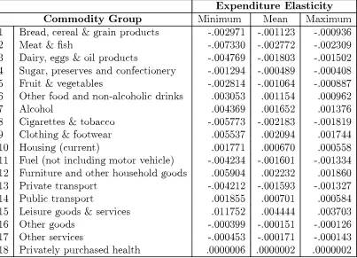
(14) COMPOSITIONAL DATA ANALYSIS AND ZEROS IN MICRO DATA. 11. and luxuries makes sense. However, the classi¯cation of Cigarettes and tobacco as a necessity is, perhaps, a little surprising until we take account of the possible addiction factor for this commodity group. We can also derive the estimated expenditure elasticities for the MAIDS model (using the estimates when ± = ±min ). This elasticity is given by: @wi @. log(Y ). =. ¯i. ¡. wi. 1 + log(Y =K ). (3.3). :. The values of the estimated elasticities, evaluated at the sample means of the wi , and for the minimum, mean and maximum values of log(Y =K ) are given in Table 6. These are all of a reasonable magnitude and are consistent with the discussion of the parameter estimates above.. Table 6: Estimated Expenditure Elasticities for Minimum, Mean and Maximum Values of log(Y K). Expenditure Elasticity Commodity Group Minimum Mean Maximum =. 1 2 3 4 5 6 7 8 9 10 11 12 13 14 15 16 17 18. Bread, cereal & grain products Meat & ¯sh Dairy, eggs & oil products Sugar, preserves and confectionery Fruit & vegetables Other food and non-alcoholic drinks Alcohol Cigarettes & tobacco Clothing & footwear Housing (current) Fuel (not including motor vehicle) Furniture and other household goods Private transport Public transport Leisure goods & services Other goods Other services Privately purchased health. -.002971 -.007330 -.004769 -.001294 -.002814 .003053 .004369 -.005773 .005537 .001771 -.004234 .005904 -.004212 .001855 .011752 -.000399 -.000453 .0000006. These elasticities are estimated at the sample means for. -.001123 -.002772 -.001803 -.000489 -.001064 .001154 .001652 -.002183 .002094 .000670 -.001601 .002232 -.001593 .000701 .004444 -.000151 -.000171 .0000002. wi. -.000936 -.002309 -.001502 -.000408 -.000887 .000962 .001376 -.001819 .001744 .000558 -.001334 .001860 -.001327 .000584 .003703 -.000126 -.000143 .0000002. .. One ¯nal issue to address in this section is the question of whether the zero replacement procedure has produced discernible patterns or outliers in the residuals from the estimation. Residual diagnostics in the form of Durbin-Watson statistics do.

(15) COMPOSITIONAL DATA ANALYSIS AND ZEROS IN MICRO DATA. 12. not indicate any patterns in the residuals8. However, a full residual diagnostic analysis looking for potential outliers has not been attempted at this juncture. It should be noted that, given that only 48 observations have no zero shares, the overwhelming majority of observations have been subject to the zero replacement procedure. As a result, it is our opinion that residual analysis to ascertain whether zero replaced observations are outliers is unlikely to be productive. We, therefore, rely on the robustness of the estimates to indicate the acceptability of the procedure. 4.. Conclusions.. This paper has discussed and modi¯ed techniques for dealing with the problem of zero observations in budget share models when the stochastic speci¯cation is made using compositional data analysis methodology. Since the compositional data approach is attractive in economics, the new techniques of dealing with the problem of zeros are of interest. When the methodology is applied to Australian household expenditure data we ¯nd that the results indicate that the procedures are simple to use and yield results that are robust to the zero replacement used. Further, these results are consistent with a priori expectations. Given the success of the application of the methodology it will be interesting to see how it works with pooled time-series cross-section data.. 8 These. are available on request..

(16) COMPOSITIONAL DATA ANALYSIS AND ZEROS IN MICRO DATA. 5.. 13. References.. Aitchison, J.A., (1986), The Statistical Analysis of Compositional Data, London: Chapman Hall. Bacon-Shone, J., (1992), \Ranking Methods for Compositional Data", Applied Statistics, , 533-537.. 41. Cooper, R. J and K.R. McLaren, (1992), \An Empirically Oriented Demand System with Improved Regularity Properties", Canadian Journal of Economics, , 652-667.. 25. Fry, J.M., Fry, T.R.L. and K.R. McLaren, (1996), \The Stochastic Speci¯cation of Demand Share Equations: Restricting Budget Shares to the Unit Simplex", in press Journal of Econometrics. McLaren, K.R., Fry, J.M. and T.R.L. Fry, (1995), \A Simple Nested Test of the Almost Ideal Demand System", Empirical Economics, , 149-161.. 20. Pudney, S.E., (1989), Modelling Individual Choice: The Econometrics of Corners, Kinks and Holes, Oxford: Basil Blackwell. Rimmer, M. and A.A. Powell, (1994), \Engel Flexibility in Household Budget Studies: Non-parametric Evidence versus Standard Functional Forms", CoPS/IMPACT Paper OP-80, Monash University..

(17)

No results found