A Closed-Form Error Model of Straight Lines for Improved Data Association and Sensor Fusing

A Closed-Form Error Model of Straight Lines for

Improved Data Association and Sensor Fusing

Volker Sommer1,†*

1 _{Beuth University of Applied Sciences; [email protected]}

† Current address: Luxemburger Str. 10, D-13353 Berlin

Abstract:Linear regression is a basic tool in mobile robotics, since it enables accurate estimation of

1

straight lines from range-bearing scans or in digital images, which is a prerequisite for reliable data

2

association and sensor fusing in the context of feature-based SLAM. This paper discusses, extends and

3

compares existing algorithms for line fitting applicable also in case of strong covariances between the

4

coordinates at each single data point, which must not be neglected if range-bearing sensors are used.

5

Besides, particularly the determination of the covariance matrix is considered, which is required for

6

stochastic modeling. The main contribution is a new error model of straight lines in closed form

7

for calculating fast and reliably the covariance matrix dependent on just a few comprehensible and

8

easily obtainable parameters. The model can be applied widely in any case when a line is fitted from

9

a number of distinct points also without a-priori knowledge of the specific measurement noise. By

10

means of extensive simulations the performance and robustness of the new model in comparison to

11

existing approaches is shown.

12

Keywords:linear regression; covariance matrix; data association; sensor fusing; SLAM

13

1. Introduction

14

Contour points acquired by active sensors using sonar, radar or lidar [1], or extracted from image

15

data [2][3], are a key source of information for mobile robots in order to detect obstacles or to localize

16

themselves in known or unknown environment [4][5]. For this purpose, often geometric features are

17

extracted from raw data since in contrast to detailed contours, features are uniquely described just

18

by a limited set of parameters and their extraction works as additional filtering in order to improve

19

reliability when dealing with sensor noise and masking [6]. However, the performance of feature based

20

localization or SLAM strongly depends on exact determination of a feature vectoryfrom measured

21

raw data. Moreover, especially for data association as well as for sensor fusing not only the feature

22

parameters are needed, but also a reliable estimation of their covariance matrixRis required, which

23

encapsulates the variances of the single elements inyand their dependencies.

24

This will be obvious if one looks at the standard algorithm for updating an estimated system state

25

ˆ

xtypically by means of EKF, compare [7][8][9]: New measurementsyare plausible if their deviations

26

from expected measurements ˆy=h(x)ˆ dependent on the in general non-linear measurement model

27

h(x)ˆ is within a limited range. For exact calculation of this limit usually the Mahalanobis-metric

28

is applied, see [8][10], which considers the covariance matrixSof the innovationν = y−yˆwith 29

S=R+H·_Pˆ·HTdependent onR, the covariance matrix ˆPof the system state and usingH=∇h(x)ˆ .

30

A new measurementywill be considered to relate to an already known feature vector ˆyif its distance

31

is below a given thresholdrth withνTS−1ν < r2_th. Only in this case, the system state vector ˆx can 32

be updated by means of∆xˆ= K·νusing the Kalman-gainK =Pˆ·HT·S, again depending on the 33

covariance matrixRof the measurements, while otherwise ˆxand ˆPare expanded by the new feature.

34

Particularly in artificial environments straight lines in a plane are frequently used as features, since

35

these are defined by just two parameters and can be clearly and uniquely determined. In contrast to

36

point features, lines in images are almost independent of illumination and perspective, and a number

37

x

ϕ

y

θ

d

r

1

N

ρ

. .

y

x

d

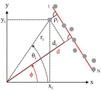
Figure 1.Parameters of measured raw data and fitted straight line

of measurements can be taken along their length to localise them accurately and to distinguish them

38

from artifacts [11]. Moreover, already a single line enables a robot to determine its orientation and

39

perpendicular distance, which clearly improves localization accuracy. Thus, many tracking systems

40

have been proposed based on line features, either using range-bearing scans [12][13] or applying visual

41

servoing, see [14][15], and also recently this approach has been successfully implemented [16][17][18].

42

However, due to missing knowledge of the covariance matrix, for data association often suboptimal

43

solutions like the Euclidian distance in Hough space [12] or other heuristics are used [19].

44

Obviously, fitting data to a straight line is a well-known technique, addressed in a large number

45

of papers [20][21][22] and textbooks [23][24][25]. In [26], a recent overview of algorithms in this field

46

is outlined. As shown in [27] and [28], if linear regression is applied to data with uncertainties in

x-47

and y-direction, always both coordinates must be considered as random variables. In [29], Arras and

48

Siegwart suggest an error model for range-bearing sensors including a covariance matrix, affected

49

exclusively by noise in radial direction. Pfister et al. introduce weights into the regression algorithm

50

in order to determine the planar displacement of a robot from range bearing scans [30]. In [31], a

51

maximum likelihood approach is used to formulate a general strategy for estimating the best fitted line

52

from a set of non-uniformly weighted range measurements. Also merging of lines and approximating

53

the covariance matrix from an iterative approach is considered. In [27] Krystek and Anton point out

54

that the weighting factors of the single measurements depend on the orientation of a line, which

55

therefore can only be determined numerically. This concept has been later extended to the general case

56

with covariances existing between the coordinates of each data point [32].

57

Since linear regression is sensitive with respect to outliers, split-and-merge algorithms must be

58

applied in advance, if a contour consists of several parts, see [33,34]. In cases of strong interference,

59

straight lines can still be identified by Hough-transformation, compare [35–37], or alternatively

60

RANSAC algorithms can be applied, see [38,39]. Although these algorithms work reliably, exact

61

determination of line parameters and estimating their uncertainties still requires linear regression [40].

62

In spite of a variety of contributions in this field, there is missing a straightforward but yet

63

accurate algorithm for determining the covariance matrix of lines reliably, fast and independently of

64

the a-priori mostly unknown measurement noise. In chapter4such a model in closed-form is proposed

65

depending on just a few clearly interpretable and easily obtainable parameters. Beforehand, in the next

66

two paragraphs existing methods for linear regression and calculation of the covariance matrix are

67

reviewed with certain extensions focussing on the usage of range-bearing sensors, which cause strong

68

covariances between x- and y-coordinates. Based on these theoretical foundations paragraph5exhibits

69

detailed simulation results in order to compare precision and robustness of the presented algorithms.

2. Determination of accurate line parameters

71

In 2d-space each straight line is uniquely described by its perpendicular distancedfrom origin

72

and by the angleφbetween positive x-axis and this normal line, see fig. 1. In order to determine 73

these two parameters, the mean squared error MSEconsidering the perpendicular distances of N

74

measurement points from the fitted line needs to be minimized. For this purpose, each perpendicular

75

distanceρiof pointiis calculated either from polar or withxi =ricosθiandyi =risinθialternatively

76

in cartesian coordinates as:

77

ρi=di−d=ricos(θi−φ)−d=xicosφ+yisinφ−d (1)

Then,MSEis defined as follows dependent onφandd: 78

MSE(φ,d) =

N

∑

i=1

(siρi)2 (2)

In (2) optional scaling valuessiare included in order to consider an individual reliability of each

79

measurement point. By calculating the derivatives of (2) with respect toφanddand setting both to 80

zero, the optimum values of these parameters can be analytically derived assuming allsito be constant,

81

i.e. independent ofφandd. The solution has been published elsewhere, compare [29], yielding forφ 82

andd:

83

φ= 1

2·atan2

−2σxy,σ_y2−σ_x2

(3)

d=x¯cosφ+y¯sinφ (4)

The function atan2() means the four quadrant arc tangent, which calculatesφalways in the 84

correct range. Ifdbecomes negative, its modulus must be taken and the correspondingφhas to be 85

altered by plus or minusπ. In these equations, ¯xand ¯ydenote the mean values of allNmeasurements 86

xiandyi, whileσx2,σy2andσxydenote the variances and the covariance:

87

σ_x2= 1

N N

∑

i=1

wi(xi−x)¯ 2 (5)

σ_y2= 1

N N

∑

i=1

wi(yi−y)¯ 2 (6)

σxy= 1 N

N

∑

i=1

wi(xi−x) (y¯ i−y)¯ (7)

¯

x= 1 N

N

∑

i=1

wixi (8)

¯

y= 1 N

N

∑

i=1

wiyi (9)

In (5) - (9), normalized weighting factors wi are used with N1 ∑iN=1wi = 1 and 0 ≤ wi ≤ 1,

88

calculated dependent on the chosen scaling valuessi:

89

wi= s

2 i 1 N∑

N i=1s2i

(10)

For convenience, in the attachment a straightforward derivation ofdandφaccording to (3) and 90

(4) is sketched.

. .

ρ

σ

σ

σ

.

ϕ

i i

i

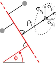
Figure 2.Optimum setting of weighting parameter for each data point

As pointed out in [32], for accurate line matching the scaling valuessimust not be assumed to

92

be constant since in general they depend onφ. This can be understood from fig.2, which shows for 93

one measurement pointithe error ellipse spanned by the standard deviationsσx,iandσy,i, while the

94

rotation of the ellipse is caused by the covarianceσxy,i.

95

Apparently, as a measure of confidence only the deviationσρ,iperpendicular to the line is relevant,

96

while the variance of any data point in parallel to the fitted line does not influence its reliability. Thus,

97

the angleφgiven in (3) will only be exact, if the error ellipse equals a circle, which means that all 98

measurements exhibit the same standard deviations inx−as iny−direction and no covariance exist.

99

Generally, in order to determine optimum line parameters with arbitrary variances and covariance of

100

each measurementi, in equation (2) the inverse ofσ_ρ,idependent onφhas to be used as scaling factor 101

si, yielding:

102

MSE(φ) =

N

∑

i=1

ρ2_i(φ)

σ_ρ2_,i(φ) (11)

In this formula, which can only be solved numerically, the varianceσ_ρ2_,ineeds to be calculated 103

dependent on the covariance matrix of each measurement point i. In case of line fitting from

104

range-bearing scans, the covariance matrix Rrθ,i can be modeled as a diagonal matrix since both 105

parametersriandθiare measured independently and thus their covarianceσrθ,iequals zero: 106

Rrθ,i=

σ_r2_,i 0

0 σ_θ2_,i

!

(12)

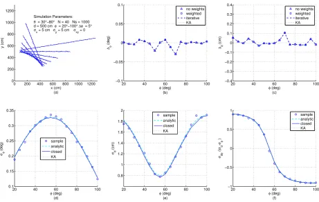
Typically, this matrix may also be considered as constant, thus independent of indexi, assuming

107

that all measured radii and angles are affected by the same noise, i.e.Rrθ,i ≈Rrθ. 108

With known variancesσ_r2_,iandσ_θ2_,iand for a certainφ, nowσ_ρ2_,iis determined by evaluating the 109

relation betweenρiand the distancesdiof each data point with 1≤i≤N. According to (1) and with

110

the distancedwritten as mean of alldiit follows:

111

ρi =di− 1 N

N

∑

j=1 dj=

_N−

1

N

di− 1

N N

∑

j=1

(j6=i)

dj (13)

Since noise induced variations of all distancesdiare uncorrelated to each other, now the variance

112

σ_ρ2_,iis calculated by means of summing over all variancesσ_d2_,i: 113

σ_ρ2_,i =

N−1

N

2

σ_d2_,i+ 1

N2 N

∑

j=1

(j6=i)

In order to deriveσ_d2_,i, changes ofdi with respect to small deviations of ri andθi from their

114

expected values ¯riand ¯θiare considered withdi=d¯i+∆di,ri =r¯i+∆riand withθi =θ¯i+∆θi:

115

∆di=∆d_ir+∆dθ

i (15)

The terms on the right side of (15) can be determined independently of each other, since∆riand

116

∆θiare assumed to be uncorrelated. Withdi=ri·cos(θi−φ)it follows 117

∆d_ir=∆ri·cos(θ¯i−φ) (16)

and

118

∆dθ i =r¯i

cos(θ¯i−φ+∆θi)−cos(θ¯i−φ)≈ −r¯i

"

∆θ2_i

2 cos(θ¯i−φ) +∆θisin(θ¯i−φ) #

(17)

In the last line the addition theorem was applied for cos(θ¯i−φ+∆θi), and for small variations

119

the approximations cos(∆θi)≈1−∆θ

2

i

2 and sin(∆θi)≈∆θiare valid.

120

The random variables∆riand∆θi are assumed to be normally distributed with variancesσ_r2_,i 121

andσ_θ2_,i. Thus, the random variable∆θ_i2exhibits aχ2-distribution with variance 2(σ_θ2_,i)2, see [41], and 122

the variance ofdiis calculated from (15), (16) and (17) as weighted sum with ¯riand ¯θiapproximately

123

replaced byriandθi, respectively:

124

σ_d2_,i= σ_r2_,i+

(σ_θ2_,i)2

2 !

cos2(θi−φ) +σ_θ2_,isin2(θi−φ) (18)

When applying this algorithm, a one-dimensional minimum search ofMSEaccording to (11)

125

needs to be executed, yielding the optimumφof the straight line. For this purpose,σ_ρ2_,iis inserted 126

from (14) considering (18), andρiis determined according to (1) by calculatingdfrom (4), (8), (9) and

127

(10) withsi =1/σ_ρ,i.

128

Obviously, numerical line fitting can also be accomplished if measurements are available in

129

cartesian coordinatesxiandyi. In this case, the covariance matrixRxy,iof each measurement point

130

must be known, defined as:

131

Rxy,i=

σ_x2_,i σxy,i

σxy,i σ_y2_,i

!

(19)

Furthermore, the partial derivatives ofdi according to (1) with respect toxi andyi need to be

132

calculated:

133

J_d,i = ∂di ∂xi

∂di ∂yi

= cosφ sinφ

(20)

Then,σ_d2_,ifollows dependent onR_xy,iandJ_d,i: 134

σ_d2_,i =J_d,i·Rxy,i·(J_d,i)T=σ_x2_,icos2φ+σxy,isinφcosφ+σ_y2_,isin2φ (21)

If raw data stems from a range-bearing scan,R_xy,ican be calculated fromR_rθ,iby exploiting the

135

known dependencies between the polar- and cartesian plane. For this purpose the Jacobian matrix

136

J_xy,iis determined:

137

J_xy,i =





∂xi ∂ri

∂xi ∂θi

∂yi ∂ri

∂yi ∂θi



=

cosθi −risinθi

sinθi ricosθi

!

Then, the covariance matrixRxy,iwill depends onRrθ,i, if small deviations from the mean value 138

of the random variablesriandθiand a linear model are assumed:

139

Rxy,i= J_xy,i·Rrθ,i·(Jxy,i)

T ₍₂₃₎

According to (23) generally a strong covarianceσxy,iinRxy,imust be considered, if measurements

140

are taken by range-bearing sensors.

141

By means of applying (21) to (23) instead of (18) for searching the minimum ofMSEdependent on

142

φ, the second order effect regarding∆θi is neglected. This yields almost the same formula as given

143

in [32], though the derivation differs and in [32] additionally the variance ofdis ignored assuming

144

σ_ρ2_,i =σ_d2_,i, which according to (14) is only asymptotically correct for largeN. 145

Finally, it should be noted that the numerical determination ofφaccording to (11) means clearly 146

more complexity compared to the straightforward solution according to equation (3). Later, in chapter

147

5it will be analyzed under which conditions this additional computational effort actually is required.

148

3. Analytic error models of straight lines

149

In literature several methods are described to estimate errors of φ and d and their mutual 150

dependency. Thus, the covariance matrixRdφmust be known, defined as: 151

R_dφ= σ 2 d σdφ σdφ σ

2

φ

!

(24)

For this purpose, a general method in nonlinear parameter estimation is the calculation of the

152

inverse Hessian matrix at the minimum ofMSE. Details can be found in [27] and [32], while in [42] it

153

is shown that this procedure may exhibit numerical instability. In section5, results using this method

154

are compared with other approaches.

155

Alternatively, in [29] and [43] an analytic error model is proposed based on fault analysis of the

156

line parameters. In this approach, the effect of variations of each single measurement point defined by

157

Rxy,iwith respect to the covariance matrix of the line parametersRdφis considered, based on (3) and 158

(4). Thereto, the Jacobian matrixJ_d

φ,iwith respect toxiandyiis determined, defined as:

159

J_d φ,i=





∂d ∂xi

∂d ∂yi ∂φ ∂xi

∂φ ∂yi



 (25)

With this matrix the contribution of a single data pointito the covariance matrix betweendandφ 160

can be written as:

161

Rdφ,i =Jdφ,i·Rxy,i·J T

dφ,i (26)

For determining the partial derivatives ofdin (25), equation (4) is differentiated after expanding

162

it by (8) and (9), yielding:

163

∂d ∂xi =wi

cosφ

N + (y¯cosφ−x¯sinφ)

∂φ

∂xi (27)

∂d ∂yi =wi

sinφ

N + (y¯cosφ−x¯sinφ)

∂φ

∂yi (28)

Differentiatingφaccording to (3) with respect toxigives the following expression withu=−2σxy

164

andv=σ_y2−σ_x2: 165

∂φ

∂xi

= 1

2(u2_+v2₎

∂u ∂xi

v− ∂v

∂xi u

The partial derivation ofuin (29) is calculated after expanding it with (7) and (8) as:

166

∂u ∂xi

=−2

N·

∂

∂xi N

∑

i=1

wixiyi−y¯

N

∑

i=1 wixi

!

=−2wi

N (yi−y)¯ (30)

while partial derivation ofvwith (5), (6) and (8) yields:

167

∂v ∂xi =−

1

N·

∂

∂xi





N

∑

i=1 wix2i −

1

N N

∑

i=1 wixi

!2

=−

2wi

N (xi−x)¯ (31)

Finally, after substituting all terms withuandvin (29) it follows:

168

∂φ

∂xi =wi

σ_x2−σ_y2

(yi−y)¯ −2σxy(xi−x)¯ N

σ_x2−σ_y2

2

+4σ_xy2

(32)

Correspondingly, for the partial derivative ofφwith respect toyithe following result is obtained:

169

∂φ

∂yi =wi

σx2−σy2

(xi−x) +¯ 2σxy(yi−y)¯ N

σ_x2−σ_y2

2

+4σ_xy2

(33)

Now, after inserting (27), (28), (32) and (33) into (25) the covariance matrix ofdandφ(24) is 170

calculated by summing over allNdata points since the noise contributions of the single measurements

171

can be assumed to be stochastically independent of each other:

172

Rdφ= N

∑

i=1 Rdφ,i=

N

∑

i=1 J_d

φ,i·Rxy,i·J T

dφ,i (34)

Equation (34) enables an exact calculation of the variancesσ_d2,σ_φ2and of the covarianceσdφas 173

long as the deviations of the measurements stay within the range of a linear approach, and as long as

174

equations (3) and (4) are valid. In contrast to the method proposed in [32] no second derivatives and

175

no inversion of the Hessian matrix are needed and thus more stable results can be expected.

176

However, both algorithms need some computational effort especially for a large number of

177

measurement points. Moreover, they do not allow to understand the effect of changing parameters

178

onRdφ, and these models can only be applied, if for each data point the covariance matrixRxy,iis

179

available. Unfortunately, for lines extracted from images this information is unknown, and also in

180

case of using range-bearing sensors just a worst case estimate ofσris given in data sheet whileσ_θis 181

ignored.

182

4. Closed-form error model of a straight line

183

In this section a simplified error model in closed form is deduced, which enables a fast, clear and

184

yet for most applications sufficiently accurate calculation of the covariance matrix R_dφin any case

185

when line parametersdandφhave been determined from a number of discrete data points. 186

Thereto, first the expected values of the line parametersdandφ, denoted as ¯dand ¯φ, are assumed 187

to be known according to the methods proposed in section2with ¯d ≈ dand ¯φ ≈ φ. Besides, for 188

modeling the small deviation ofdandφ, the random variables∆dand∆φare introduced. Thus, with 189

d=d¯+∆dandφ=φ¯+∆φit follows for the variances and the covariance: 190

θ₁

x

L

ϕ θN

Δd

d

xoff

Δϕ

ρ

∼

_ _

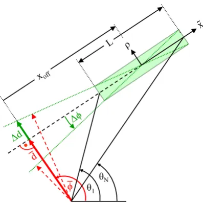
Figure 3.Dependency between∆d,∆φand geometric parameters

x L

i=−N

2 i=

N

2

Δx

Figure 4.Details of fig.3with the deviation of data points along the axis ˜x

Next,∆dand∆φshall be determined dependent on a random variation of any of theNmeasured 191

data points. For this purpose, fig.3is considered, which shows the expected line parameters and the

192

random variables∆dand∆φ. 193

In order to derive expressions for∆dand∆φdepending on the random variablesρi, fig.4shows

194

an enlargement of the rectangular box depicted in fig.3along the direction of the line ˜x.

195

First, the effect of variations of anyρion∆φis considered. Since∆φis very small, this angle may 196

be replaced by its tangent, which defines the slope∆mof the line with respect to the direction ˜x. Here,

197

onlyρiis considered as a random variable but not ˜xi. Thus, the standard formula for the slope of a

198

regression line can be applied, which will minimize the mean squared distance in the direction ofρ, if 199

all ˜xiare assumed to be exactly known:

200

∆φ≈tan(∆φ) =∆m= σρx˜ σ_x2_˜

= ∑

i

ρi·xi˜ ∑

i

˜

x2 i

(36)

Now, in order to calculate the variance of∆φ, a linear relation between∆φand eachρiis required,

201

which is provided by the first derivation of (36) with respect toρi:

202

∂∆φ

∂ρi = xi˜

∑ i

˜

x2_i (37)

Then, the variance of∆φdependent on the variance ofρican be specified. From (37) it follows:

σ_∆2_φ,i =σ_ρ2_,i·

∂∆φ

∂ρi

2

=σ_ρ2_,i· x˜

2 i

∑ i

˜

x2_i

2 (38)

Ifσ_ρ2_,i is assumed to be approximately independent ofi, it may be replaced byσ_ρ2and can be 204

estimated from (2) withρitaken from (1) and setting allsito 1/N:

205

σ_ρ2_,i≈σ_ρ2= 1

N N

∑

i=1

ρi(φ,d)2 (39)

It should be noted, that for a bias-free estimation ofσ_ρ2with (39), the exact line parametersφandd 206

must be used in (1), which obviously are not available. If instead estimated line parameters according

207

to chapter2are taken, e. g. by applying (3) and (4), calculated from the same data as used in (39),

208

an underestimation ofσ_ρ2especially for small Ncan be expected, sinceφanddare determined by 209

minimizing the variance ofρof theseNdata points. This is referred to later. 210

Next, from (38) the variance of∆φresults as sum over allNdata points, since allρiare independent

211

of each other:

212

σ_∆2_φ=

∑

i

σ_∆2_φ,i≈σ_ρ2· ∑

i

˜

x_i2

∑ i

˜

x2_i

2 =σ

2

ρ·

1

∑ i

˜

x2_i (40)

Equation (40) with (35) and (39) enables an exact calculation ofσ_φ2dependent on theNdata points 213

of the line.

214

However, from (40) a straightforward expression can be derived, which is sufficiently accurate in

215

most cases and enables a clear understanding of the influencing parameters onσ_φ2, compare section5. 216

For this purpose, according to fig.3the lengthLof a line segment is determined from the perpendicular

217

distancedand from the anglesθ1andθNof the 1stand Nthdata point, respectively:

218

L=d· |tan(φ−θN)−tan(φ−θ1)| (41)

Furthermore, a constant spacing∆x˜between adjacent data points is assumed:

219

∆x˜≈ L

N−1. (42)

Applying this approximation, the sum over all squared ˜xican be rewritten, yielding for evenNas

220

depicted in fig.4:

221

∑

i

˜

x2_i ≈2·

N/2

∑

i=1

_∆

˜

x

2 (2i−1)

2

=∆x˜2·

N/2

∑

i=1

(2i−1)2

2 (43)

The last sum can be transformed into closed form as:

222

N/2

∑

i=1

(2i−1)2

2 =

N 2

4N₂2−1

6 =

N(N2−1)

12 (44)

WithNodd, the sum must be taken twice from 1 toN−₂1since in this case the central measurement

223

point has no effect onσ_∆2_φ,i, yielding: 224

∑

i

˜

x2_i ≈2·

(N−1)

2

∑

i=1

[∆x˜·i]2=∆x˜2· (N−1)

2

∑

i=1

Again, the last sum can be written in closed form, which gives the same result as in (44):

225

(N−1) 2

∑

i=1

2·i2= N−1

2

_N−

1

2 +1 2· N−1

2 +1

3 =

N(N2−1)

12 (46)

Finally, by substituting (43) with (44), or (45) with (46) into (40) and regarding (35) as well as (42),

226

a simple analytic formula for calculating the variance ofφis obtained, just depending onL,Nand the 227

variance ofρ: 228

σ_φ2≈σ_ρ2· 12

L2_·N· N−1

N+1

N1

≈ σ_ρ2· 12

L2_·N (47)

The last simplification in (47) overestimatesσ_φ2a little bit for smallN. Interestingly, this error 229

compensates quite well for a certain underestimation ofσ_ρ2according to (39), assuming that the line 230

parametersφanddare determined from the same data asσ_ρ2, see chapter5. 231

Next, in order to deduce the varianceσ_d2, again fig. 3is considered. Apparently, a first part of 232

the random variable∆dis strongly correlated to∆φsince any mismatch inφis transformed into a 233

deviation∆dby means of the geometric offsetxo f f with:

234

∆dφ_=−x

o f f ·∆φ (48)

Actually, with a positive value forxo f f as depicted in fig.3the correlation between∆dand∆φ 235

becomes negative, since positive values of∆φcorrespond to negative values of∆d. According to fig.3, 236

xo f f is determined fromφanddas well as fromθ1andθN:

237

xo f f = d

2·[tan(φ−θN) +tan(φ−θ1)] (49)

Alternatively,xo f f can be taken as mean value from allNdata points of the line segment:

238

xo f f = d N ·

N

∑

i=1

tan(φ−θi) (50)

Nevertheless, it should be noted that∆dis not completely correlated with∆φ, since also in the 239

casexo f f =0 the error∆dwill not be zero.

240

Indeed, as a second effect each singleρihas a direct linear impact on the variable∆d. For this purpose,

241

in fig.4the random variable∆dρ_{is depicted, which describes a parallel shift of the regression line due} 242

to variation inρi, calculated as mean value over allρi:

243

∆dρ₌ 1

N·

∑

Combining both effects, variations indcan be described as the sum of two uncorrelated terms,

244

∆dφ_and∆_dρ_: 245

∆d=∆dφ₊∆_dρ_{=−xo f f ·}∆_φ+ 1

N ·

∑

This missing correlation between∆φand the sum over allρiis also intuitively accessible: If the

246

latter takes a positive number it will not be possible to deduce the sign or the modulus of∆φ. From 247

(52) and withE(∆dφ_·∆_dρ_{) =0,E(}∆_dφ_{) =0 andE(}∆_dρ_{) =0 the varianceσ}2

dcan be calculated as

248

σ_d2=E([∆d]2) =E([∆dφ]2) +E([∆dρ]2) =x2_{o f f} ·E([∆φ]2) + 1

N2·E



 "

∑

i

ρi

#2

0 200 400 600 800 1000 1200 0

200 400 600 800 1000 1200

Simulation Parameters:

d = 500 cm φ = 20°−100° ∆φ = 5°

θ = 30°−80° N = 40 Ns = 1000

σ

x = 5 cm σy = 5 cm σxy = 0

x (cm) (a)

y (cm)

20 40 60 80 100

−0.1 −0.05 0 0.05 0.1

φ (deg) (b)

∆φ

(deg)

no weights weighted iterative KA

20 40 60 80 100

−0.4 −0.3 −0.2 −0.1 0 0.1 0.2 0.3 0.4

φ (deg) (c)

∆d

(cm)

no weights weighted iterative KA

20 40 60 80 100

0.1 0.15 0.2 0.25 0.3 0.35

φ (deg) (d)

σφ

(deg)

sample analytic closed KA

20 40 60 80 100

0.8 1 1.2 1.4 1.6 1.8 2

φ (deg) (e)

σd

(cm)

sample analytic closed KA

20 40 60 80 100

−1 −0.5 0 0.5 1

φ (deg) (f)

σd

φ

/(

σd ⋅σφ

)

sample analytic closed KA

Figure 5.Simulation Results for equidistant measurement points superimposing normal distributed

and uncorrelated noise inx- andy-direction

≈x2_{o f f} ·σ_φ2+ 1

N·σ 2

ρ (54)

In the last step from (53) to (54) again the independence of the single measurements from each

249

other is used, thus the variance of the sum of theNdata points approximatesN-times the varianceσ_ρ2. 250

Finally, the covariance betweenφanddneeds to be determined. Based on the definition it follows 251

withσdφ=σ∆d∆φ 252

σ_dφ=E(∆d·∆φ) =E(∆dφ·∆φ) +E(∆dρ·∆φ) =−x_{o f f} ·E([∆φ]2) =−x_{o f f}·σ_φ2 (55)

By means of (47), (54) and (55), now the complete error model in closed form is known, represented

253

by the covariance matrixR_dφgiven as:

254

R_dφ≈σ_ρ2·



 

12·x2

o f f L2_·N +N1

−12·x_{o f f} L2_·N

−12·x_{o f f}

L2_{·N L}122_·N 



 (56)

Applying this error model is easy since no knowledge of the variances and covariance for each

255

single measurement is needed, which in practice is difficult to acquire. Instead, just the numberNof

256

preferably equally spaced points used for line fitting, the lengthLof the line segment, its offsetxo f f

257

and the varianceσ_ρ2according to (41), (49) and (39) must be inserted. 258

5. Simulation results

259

The scope of this section is to compare the presented algorithms for linear regression and

260

error modeling based on statistical evaluation of the results. Segmentation of raw data is not

261

considered; if necessary this must be performed beforehand by means of well-known methods

like Hough-Transformation or RANSAC, compare section1. Thus, for studying the performance

263

reliably and repeatably, a large number of computer simulations was performed, applying a systematic

264

variation of parameters within a wide range, which would not be feasible if real measurement are

265

used.

266

For this purpose, straight lines with a certain perpendicular distancedfrom origin and within

267

a varying range of normal anglesφhave been specified. Each of these lines is numerical described 268

by a number ofNpoints either given in cartesian (xi,yi) or in polar (riθi) coordinates. In order to

269

simulate the outcome of a real range-bearing sensor as close as possible, the angular coordinate was

270

varied betweenθ1andθN. To each measurement a certain amount of normally distributed noise with

271

σx,σyandσxyor alternatively withσrandσ_θwas added. Further, for eachφa number ofNs=1000 272

sets of samples was generated, in order to allow statistical evaluation of the results. A first simulation

273

was performed withN = 40 equally spaced points affected each by uncorrelated noise inx−and

274

y−direction with standard deviationsσx=σy=5cm. This is a typical situation when a line is calculated

275

from binary pixels, and in subfigure (a) of fig. 5a bundle of the simulated line segments is shown.

276

The deviations∆φand∆dtaken as mean value over all Ns samples of the estimatedφandd from 277

their true values, respectively, are depicted in subfigures (b) and (c) comparing four algorithms as

278

presented in section2: The triangles mark the outcome of equations (3) and (4) with all weights set to

279

one, whereas the squares are calculated according to the same analytic formulas but using individual

280

weighting factors applying (10) withsi = 1/σ_ρ,i. The perpendicular deviationsσ_ρ,iare determined

281

according to (14) and (21) withφ taken from (3) without weights. Obviously, in this example all 282

triangles coincide with the squares since each measurementiis affected by the same noise and thus

283

for anyφall weighting factors are always identical. The dashed lines in (b) and (c) show the results 284

when applying the iterative method according to (11) with the minimum ofMSEfound numerically.

285

For this purpose,σ_ρ2_,iis inserted from (14) considering (21),ρiis taken from (1) anddis calculated from

286

(4), (8), (9) and (10) withsi =1/σ_ρ,i. The dotted lines (KA) depict the deviations ofdandφobtained 287

according to Krystek and Anton in [32]. Both numerical algorithm yield the same results, which is

288

not surprising, since the variancesσ_ρ2_,iused as weighting factors are all identical. Further, here the 289

analytical algorithms provide exactly the same performance as the numerical ones, since forσx=σy

290

the weighting factors show no dependency onφand for that case the analytical formulas are optimal. 291

The lower subfigures depict the parameters of the covariance matrixRdφ again as a function 292

ofφcomparing different methods. Here, the circles represent numerical results obtained from the 293

definitions of variance and covariance by summing over allNspasses with 1≤k≤Ns, yieldingdkand

294

φk, respectively:

295

σ_d2= 1

Ns Ns

∑

k=1

(dk−d)2 (57)

σ_φ2= 1

Ns Ns

∑

k=1

(φk−φ)2 (58)

σ_dφ= 1

Ns Ns

∑

k=1

(dk−d) (φk−φ) (59)

Since these numerical results serve just as reference for judging the accuracy of the error models,

296

in the formulas above the true values fordandφhave been used. The required line parametersdk 297

andφ_kin (57) - (59) can be estimated with any of the described four methods, since minor differences 298

indkandφk have almost no effect on the resulting variances and the covariance. The dashed lines

299

in subfigures (d) - (f) show the results of the analytic error model as described in section3, and

300

the dotted lines represent the outcomes of the algorithm from Krystek and Anton [32], while the

301

continuous line corresponds to the model in closed-form according to (56) in section4withLand

302

xo f f taken from (41) and (49), respectively. Interestingly, although the theoretical derivations differ

2 4 6 8 10 12 14 16 18 20 0

5 10 15 20 25 30

Number N of measurement points

σ ρ 2 (cm 2 )

with exact line parameters with estimated line parameters estimated with correction

Figure 6.Variance ofρdependent on the numberNof measured data points, using the same simulation

parameters as indicated in figure5(a)

substantially, the results match very well, which especially proves the correctness of the simplified

304

model in closed-form. Since this model explicitly considers the effect of the line lengthLand of the

305

geometric offsetxo f f, the behavior of the curves can be clearly understood: The minimum ofLwill

306

occur ifφequals the mean value ofθminandθmax, i.e. atφ=55◦, and exactly at this angle the maximum 307

standard deviationσφoccurs. Further, sinceLlinearly depends onφ, a quadratic dependence ofσφ 308

onφaccording to (47) can be observed. With respect to fig.5(e) the minimum ofσdalso appears at

309

φ=55◦corresponding tox_{o f f} =0. At this angle according to (54) the standard deviation ofdis given 310

asσ_d≈σρ/

√

N=5/√40=0.79, while the covarianceσ_ρdcalculated according to (55) and with it the 311

correlation coefficient shown in fig.5(f) vanishes.

312

When comparing the results, one should be aware that in the simulations of the analytic error

313

models the exact variancesσ_x2_i,σ_y2_i andσxy_i are used, thus in practice achievable accuracies will be

314

worse. On the other hand, when applying the new error model in closed-form, the varianceσ_ρ2is 315

calculated as mean value of allρ2_i from the actual set ofNdata points according to (39) and hence is 316

always available.

317

Nevertheless, if in this equation the estimated line parametersφand d are used, which are 318

calculated e. g. according to (3) and (4) using the same measurements as in (39), no unbiasedσ_ρ2can 319

be expected. This is reasoned from the fact that for each set ofNdata points, the mean quadratic

320

distance over allρ2_i is minimized in order to estimateφandd. Thus, the numeric value ofσ_ρ2will 321

always be smaller than its correct value calculated with the exact line parameters. This effect can be

322

clearly observed from fig.6, which shows for the same simulation parameters as depicted in fig.5(a)

323

the dependency ofσ_ρ2on the number of points on the lineN, averaged overNssets of samples: Only 324

in case of using the exact line parameters in (39), which obviously are only available in a simulation,

325

actually the correctσ_ρ2 =25cm2is obtained as shown by the triangles. If however at each runσ_ρ2is 326

calculated with the estimatedφanddas indicated by the squares, a clear deviation especially at lowN 327

occurs. Only asymptotically for largeNwhenφconverges to its exact value the correctσ_ρ2is reached. 328

Fortunately, this error can be compensated quite well by means of multiplyingσ_ρ2with a correction 329

factorc= N_N−+1₁as shown by the dashed line in fig.6. Due to the strongly non-linear relation betweenφ 330

and anyρi, this correction works much better than simply exchanging in (39) the divisorNbyN−1

331

0 200 400 600 800 1000 1200 0

200 400 600 800 1000 1200

Simulation Parameters:

d = 500 cm φ = 20°−100° ∆φ = 5°

θ = 30°−80° N = 40 Ns = 1000

σ

r = 5 cm σθ = 0.1° σrθ = 0

x (cm) (a)

y (cm)

20 40 60 80 100

−0.04 −0.03 −0.02 −0.01 0 0.01 0.02 0.03

φ (deg) (b)

∆φ

(deg)

no weights weighted iterative KA

20 40 60 80 100

−0.1 −0.05 0 0.05 0.1 0.15 0.2 0.25

φ (deg) (c)

∆d

(cm)

no weights weighted iterative KA

20 40 60 80 100

0.05 0.1 0.15 0.2 0.25 0.3 0.35 0.4

φ (deg) (d)

σφ

(deg)

sample analytic closed KA

20 40 60 80 100

0.7 0.8 0.9 1 1.1 1.2 1.3 1.4 1.5

φ (deg) (e)

σd

(cm)

sample analytic closed KA

20 40 60 80 100

−1 −0.5 0 0.5 1

φ (deg) (f)

σd

φ

/(

σd ⋅σφ

)

sample analytic closed KA

Figure 7.Results from simulated range-bearing scans superimposing low noise inr- andθ-direction

(47), the closed-form of the covariance matrixRdφaccording to (56) yields almost unbiased results also 333

for smallNifσ_ρ2is calculated according to (39) with estimated line parametersφandd. Although not 334

shown here, the proposed bias compensation works well for a large range of measurement parameters.

335

For a reliable determination ofσ_ρ2fromNdata points of a line segment,Nshould be at least in the 336

order of 10.

337

Figure7shows the results when simulating a range-bearing scan with a constant angular offset

338

∆θ = (θmax−θmin)/(N−1) between adjacent measurements. Each measurement is distorted by

339

adding normally distributed noise with standard deviationsσr=5cmandσ_θ =0.1◦. This is a more 340

challenging situation, since now the measurements are not equispaced, each data point exhibits

341

individual variancesσx,i,σy,idependent onφ, and moreover a covarianceσxy,iexists. As can be seen,

342

the errors of the estimatedφand das depicted in subfigure (b) and (c) exhibit the same order of 343

magnitude as before, yet, both analytic results differ slightly from each other and are less accurate

344

compared to the numerical solutions. Both numerical methods yield quasi identical results, since for

345

the chosen small noise amplitudes the differences between both algorithms have no impact on the

346

resulting accuracy.

347

Regarding the error models, subfigures (d) to (f) reveal, that in spite of unequal distances between

348

the measurement points and varyingσρ,ithe results of the closed-form model match well with the

349

analytic and numeric results. Onlyσdshows a certain deviation at steep and flat lines withφbelow 30◦ 350

or above 80◦. This is related to errors inxo f f, since in this range ofφthe points on the lines measured 351

with constant∆θhave clearly varying distances and thus (49) yields just an approximation of the 352

effective offset of the straight line.

353

The next figure8shows the results with the models applied to short lines measured in the angular

354

range of 30◦≤θ≤40◦withN=20, while all other parameters are identical to those depicted in fig. 355

7(a). As can be seen from subfigures (b) and (c), now the analytical algorithms based on (3) and (4)

356

are no longer adequate since these, independent of applying weights or not, yield much higher errors

0 200 400 600 800 1000 1200 0 200 400 600 800 1000 1200 Simulation Parameters:

d = 500 cm φ = 20°−100° ∆φ = 5°

θ = 30°−40° N = 20 Ns = 1000

σ

r = 5 cm σθ = 0.1° σrθ = 0

x (cm) (a)

y (cm)

20 40 60 80 100

−0.5 −0.4 −0.3 −0.2 −0.1 0 0.1 0.2 0.3 0.4

φ (deg) (b) ∆φ (deg) no weights weighted iterative KA

20 40 60 80 100

−1 −0.5 0 0.5 1 1.5 2 2.5

φ (deg) (c) ∆d (cm) no weights weighted iterative KA

20 40 60 80 100

0 0.5 1 1.5 2 2.5

φ (deg) (d) σφ (deg) sample analytic closed KA

20 40 60 80 100

1 2 3 4 5 6 7 8 9

φ (deg) (e) σd (cm) sample analytic closed KA

20 40 60 80 100

−1 −0.5 0 0.5 1

φ (deg) (f) σd φ /( σd ⋅σφ ) sample analytic closed KA

Figure 8.Results from simulated range-bearing scans of short lines superimposing low noise inr- and

θ-direction

0 200 400 600 800 1000 1200 0 200 400 600 800 1000 1200 Simulation Parameters:

d = 500 cm φ = 20°−100° ∆φ = 5°

θ = 30°−80° N = 20 Ns = 1000

σ

r = 0 cm σθ = 2° σrθ = 0

x (cm) (a)

y (cm)

20 40 60 80 100

−0.4 −0.3 −0.2 −0.1 0 0.1 0.2 0.3 0.4

φ (deg) (b) ∆φ (deg) no weights weighted iterative KA

20 40 60 80 100

−2 −1.5 −1 −0.5 0 0.5

φ (deg) (c) ∆d (cm) no weights weighted iterative KA

20 40 60 80 100

0.2 0.3 0.4 0.5 0.6 0.7 0.8 0.9 1

φ (deg) (d) σφ (deg) sample analytic closed KA

20 40 60 80 100

0 2 4 6 8 10 12

φ (deg) (e) σd (cm) sample analytic closed KA

20 40 60 80 100

−1 −0.5 0 0.5 1

φ (deg) (f) σd φ /( σd ⋅σφ ) sample analytic closed KA

0 200 400 600 800 1000 1200 0

200 400 600 800 1000 1200

Simulation Parameters:

d = 500 cm φ = 20°−100° ∆φ = 5°

θ = 30°−80° N = 10 Ns = 1000

σ

r = 5 cm σθ = 0.1° σrθ = 0

x (cm) (a)

y (cm)

20 40 60 80 100

−0.03 −0.02 −0.01 0 0.01 0.02 0.03 0.04

φ (deg) (b)

∆φ

(deg)

no weights weighted iterative KA

20 40 60 80 100

−0.15 −0.1 −0.05 0 0.05 0.1 0.15 0.2 0.25

φ (deg) (c)

∆d

(cm)

no weights weighted iterative KA

20 40 60 80 100

0.1 0.2 0.3 0.4 0.5 0.6 0.7 0.8 0.9

φ (deg) (d)

σφ

(deg)

sample analytic closed KA

20 40 60 80 100

1 1.5 2 2.5 3 3.5 4

φ (deg) (e)

σd

(cm)

sample analytic closed KA

20 40 60 80 100

−1 −0.5 0 0.5 1

φ (deg) (f)

σd

φ

/(

σd ⋅σφ

)

sample analytic closed KA

Figure 10. Results from simulated range-bearing scans with a low number of data points and only

approximately known noise level of the sensor

than the numerical approaches. All error models however provide still accurate results. Actually, the

358

closed-form model even yields better accuracy than before, since the distances of the data points on

359

the line between adjacent measurement and alsoσ_ρ,iare more uniform compared to the simulations

360

with long lines.

361

In order to check the limits of the models, figure9depicts the results when applying large

362

angular noise withσ_θ=2◦. In this extreme case also the numerical algorithms show systematic errors 363

dependent onφsince the noise ofρican no longer be assumed to be normally distributed. However,

364

according to subfigures (b) and (c) the iterative method as presented in section2shows clear benefits

365

in comparison to the KA-algorithm proposed in [32], caused by the more accurate modeling ofσρi.

366

With respect to the outcome of the noise models in subfigures (d) to (f), now only the analytic

367

algorithm as presented in paragraph3still yields reliable results, while the KA-method based on

368

matrix inversion reveals numerical instability. Due to the clear uneven distribution of measurements

369

along the line also the simplified error model in this case shows clear deviations, although at least the

370

order of magnitude is yet correct.

371

Finally, figure10shows typical results, if the sensor noise is not exactly known. In this example,

372

the radial standard deviation was assumed to be 10 cm whereas the exact value, applied when

373

generating the measurements, was only 5 cm. The simulation parameters correspond to those in figure

374

7, only the number of data points has been reduced toN=10. According to subfigures (b) and (c), now

375

for calculatingφanddthe numerical methods yield no benefit over the analytical formulas with or 376

without weights. Due to the only approximately known variance, the analytic error model as well

377

as the KA-method in (d) to (f) reveal clear deviations from the reference results. Only the model in

378

closed-form is still accurate, since it does not require any a-priori information regarding sensor noise.

379

In addition, these results prove the bias-free estimation ofσ_ρ2with (39) also ifNis low as depicted in 380

figure6.

6. Conclusion

382

In this study the performance of linear regression is evaluated, assuming both coordinates as

383

random variables. It is shown, that especially with range-bearing sensors, frequently used in mobile

384

robotics, a distinct covariance of the noise in x- and y-direction at each measurement point exists. In

385

this case, analytical formulas assuming identical and uncorrelated noise, will only provide accurate

386

line parametersφanddif the detected line segments are sufficiently long and the noise level stays 387

below a certain limit. If this prerequisites are not fulfilled and if the sensor noise is known, numerical

388

algorithms should be applied, which consider the reliability of each measurement point as a function

389

ofφ. At this, the performance of prior art can be improved by means of modeling the independence of 390

the single data points exactly and by paying attention also to 2nd order effects of the angular noise.

391

The main focus of this paper is on the derivation of the covariance matrixRdφof straight lines. 392

This information has crucial impact on the performance of SLAM with line features, since for both, data

393

association and sensor fusing,Rdφmust be estimated precisely. For this purpose, first analytical error 394

models are reviewed, which however need exact knowledge of the measurement noise, although in

395

many applications this is not available. In addition, these approaches require high computational effort

396

and do not allow to comprehend the effect of measurement parameters on the resulting accuracy of an

397

estimated straight line. Thus, a new error model in closed form is proposed, just depending on two

398

geometric parameters as well as on the number of points of a line segment. Besides, a single variance

399

must be known, which is determined easily and reliably from the same measurements as used for line

400

fitting. By means of this model the covariance matrix can be estimated fast and exactly. Moreover,

401

it allows to adapt measurement conditions in order to achieve maximum accuracy of detected line

402

features.

403

Appendix. Analytic derivation of straight line parameters with errors in both coordinates

404

For the derivation of the perpendicular distanced, the partial derivative of equation (2) with

405

respect todis taken and set to zero, which directly gives equation (4) using (8), (9) and (10). In order

406

to calculateφ, first the partial derivation of (2) with respect toφmust be calculated and set to zero, 407

yielding:

408

1

N N

∑

i=1 si

h

xiyi

cos2φ−sin2φ

+y2_i−x2_isinφ cosφ

i

+ 1 N

N

∑

i=1

sid(xisinφ−yicosφ) =0 (A1)

Now, the distancedcan be replaced by (4), and after inserting the definitions of ¯x, ¯y,σ2_x,σ_y2and 409

σxyaccording to (5) - (9) considering (10) it follows from (A1) after reordering:

410

σxy

cos2φ−sin2φ

+sinφcosφ

σ_y2−σ_x2

=0 (A2)

Applying the theorem ofPythagorasand the addition theorems of angles, the terms with sine and

411

cosine can be rewritten:

412

cos2φ−sin2φ=2 cos2φ−1=cos 2φ (A3)

sinφcosφ= 1

2sin 2φ (A4)

Inserting these formulas into (A2), finally yields forφ: 413

φ= 1

2arctan

−2σxy

σy2−σx2

!

(A5) calculates φalways in the range−π/4 < φ < π/4, although according to fig. 1this is 414

only correct ifσ_y2>σ_x2, while in the caseσ_y2<σ2_xan angleπ/2 must be added toφ. Thus, as general 415

solution (3) should be taken also avoiding a special consideration ifσ_y2equalsσ2_x. 416

References

417

1. Everett, H.R.Sensors for Mobile Robots; Number ISBN 978-1568810485, A. K. Peters, 1995. 418

2. Canny, J. A Computational Approach to Edge Detection. IEEE Trans. Pattern Analysis and Machine

419

Intelligence1986,8, 679–698. 420

3. Guse, W.; Sommer, V. A New Method for Edge Oriented Image Segmentation.Picture Coding Symposium,

421

Tokio1991. 422

4. Gao, Y.; Liu, S.; Atia, M.M.; Noureldin, A. INS/GPS/LiDAR Integrated Navigation System for Urban and 423

Indoor Environments Using Hybrid Scan Matching Algorithm. Sensors2015,15, 23286–23302. 424

5. Lu, F.; Milios, E. Robot pose estimation in unknown environments by matching 2D range scans. Journal of

425

Intelligent and Robotic Systems1997,18, 249–275. 426

6. Arras, K.O.; Castellanos, J.A.; Schilt, M.; Siegwart, R. Feature-based multi-hypothesis localization and 427

tracking using geometric constraints. Robotics and Autonomous Systems2003,44, 41–53. 428

7. Borenstein, J.; Everett, H.R.; Feng, L. Navigating Mobile Robots, Systems and Techniques; Number ISBN 429

978-1568810669, A. K. Peters, 1996. 430

8. Neira, J.; Tardos, J.D. Data association in stochastic mapping using the joint compatibility test. IEEE

431

Transactions on Robotics and Automation2001,17, 890–897. 432

9. Durrant-Whyte, H.; Bailey, T. Simultaneous localization and mapping: part I.IEEE Robotics & Automation

433

Magazine2006,13, 99–110. 434

10. Blanco, J.L.; Gonzalez-Jimenez, J.; Fernandez-Madrigal, J.A. An Alternative to the Mahalanobis Distance 435

for Determining Optimal Correspondences in Data Association. Transactions on Robotics2012,28, 980–986. 436

11. Wang, H.; Liu, Y.H.; Zhou, D. Adaptive Visual Servoing Using Point and Line Features With an 437

Uncalibrated Eye-in-Hand Camera. IEEE Transactions on Robotics2008,24, 843–857. 438

12. Choi, Y.H.; Lee, T.K.; Oh, S.Y. A line feature based SLAM with low grade range sensors using geometric 439

constraints and active exploration for mobile robot. Autonomous Robots2008,24, 13–27. 440

13. Yin, J.; Carlone, L.; Rosa, S.; Anjum, M.L.; Bona, B. Scan Matching for Graph SLAM in Indoor Dynamic 441

Scenarios. Proceedings of the Twenty-Seventh International Florida Artificial Intelligence Research Society

442

Conference2014, pp. 418–423. 443

14. Pasteau, F.; Narayanan, V.K.; Babel, M.; Chaumette, F. A visual servoing approach for autonomous corridor 444

following and doorway passing in a wheelchair. Robotics and Autonomous Systems2016,75, 28–40. 445

15. David, P.; DeMenthon, D.; Duraiswami, R.; Samet, H. Simultaneous pose and correspondence 446

determination using line features.Proc. of Computer Vision and Pattern Recognition2003,2, 424–431. 447

16. Marchand, É.; Fasquelle, B. Visual Servoing from lines using a planar catadioptric system. Conf. on

448

Intelligent Robots and Systems (IROS)2017, pp. 2935–2940. 449

17. Bista, S.R.; Giordano, P.R.; Chaumette, F. Combining Line Segments and Points for Appearance- based 450

Indoor Navigation by Image Based Visual Servoing. IEEE/RSJ International Conference on Intelligent Robots

451

and Systems (IROS)2017, pp. 2960–2967. 452

18. Xu, D.; Lu, J.; Wang, P.; Zhang, Z.; Liang, Z. Partially Decoupled Image-Based Visual Servoing Using 453

Different Sensitive Features.IEEE Transactions on Systems, Man, and Cybernetics: Systems2017,47, 2233–2243. 454

19. Jeong, W.Y.; Lee, K.M. Visual SLAM with Line and Corner Features. Conference on Intelligent Robots and 455

System, IROS. IEEE, 2006. 456

20. York, D. Least-squares fitting og a straight line. Can. J. Phys.1966,44, 1079–1086. 457

21. Krane, K.S.; Schecter, L. Regression line analysis.Am. J. Phys.1982,50. 458

22. Golub, G.; van Loan, C. Ana analysis of the total least squares problem. SIAM J. Num. Anal. 1980, 459

17, 883–893. 460

23. Weisberg, S.Applied linear regression, 3rd edition ed.; Number ISBN 0-471-66379-4, John Wiley & Sons, 2005. 461

24. Draper, N.R.; Smith, H.Applied Regression Analysis, 3rd edition ed.; John Wiley & Sons, 1988. 462

25. Seber, G.A.F.; Lee, A.J.Linear Regression Analysis, 2nd edition ed.; Number ISBN 0 471 41540 5, John Wiley 463

26. Amiri-Simkooeiab, A.R.; Zangeneh-Nejadac, F.; Asgaria, J.; Jazaeri, S. Estimation of straight line parameters 465

with fully correlated coordinates. Journal of the International Measurement Confederation2014,48, 378–386. 466

27. Krystek, M.; Anton, M. A weighted total least-squares algorithm for fitting a straight line.Measurement

467

Science and Technology2007,18, 3438–3442. 468

28. Cecchi, G.C. Error analysis of the parameters of a least-squares determined curve when both variables 469

have uncertainties. Measurement Science and Technology1991,2, 1127–1129. 470

29. Arras, K.O.; Siegwart, R.Y. Feature Extraction and Scene Interpretation for Map-Based Navigation and 471

Map Building. Proc. of SPIE, Mobile Robotics XII, 1997, pp. 42–53. 472

30. Pfister, S.T.; Kriechbaum, K.L.; S. I. Roumeliotis, J.W.B. A Weighted range sensor matching algorithms for 473

mobile robot displacement estimation. Proceedings IEEE International Conference on Robotics and Automation

474

2002,4.

475

31. Pfister, A.T.; Roumeliotis, S.I.; Burdick, W. Weighted line fitting algorithms for mobile robot map building 476

and efficient data representation. Proc. of the 2003 IEEE int. Conf. on Robotics and Automation2003, pp. 477

1304–1311. 478

32. Krystek, M.; Anton, M. A least-squares algorithm for fitting data points with mutually correlated 479

coordinates to a straight line. Measurement Science and Technology2011,22, 1–9. 480

33. Borges, G.A.; Aldon, M.J. A Split-and-Merge Segmentation Algorithm for Line Extraction in 2-D Range 481

Images. Proceedings. 15th International Conference on Pattern Recognition2000,4. 482

34. Jian, M.; Zhang, C.F.; Yan, F.; Tang, M.Z. A global line extraction algorithm for indoor robot mapping based 483

on noise eliminating via similar triangles rule. 35th Chinese Control Conference (CCC)2016, pp. 6133–6138. 484

35. J.Illingworth.; J.Kittler. A survey of the hough transform.Computer Vision, Graphics, and Image Processing

485

1988,44, 87–116. 486

36. Kim, J.; Krishnapuram, R. A Robust Hough Transform Based on Validity. Internat. Conf. on Computational 487

Intelligence. IEEE, 1998, Vol. 2, pp. 1530–1535. 488

37. Banjanovic-Mehmedovic, L.; Petrovic, I.; Ivanjko, E. Hough Transform based Correction of Mobile Robot 489

Orientation. Internat. Conf. on Industrial Technology2004,3, 1573–1578. 490

38. Fischler, M.A.; Bolles, R.C. Random Sample Consensus: A Paradigm for Model Fitting with Applications 491

to Image Analysis and Automated Cartography. Communications of the ACM1981,25, 381–395. 492

39. Liu, Y.; Gu, Y.; Li, J.; Zhang, X. Robust Stereo Visual Odometry Using Improved RANSAC-Based Methods 493

for Mobile Robot Localization. Sensors2017,17, 2339–2357. 494

40. Nguyen, V.; Martinelli, A.; Tomatis, N.; Siegwart, R. A Comparison of Line Extraction Algorithms using 495

2D Laser Rangefinder for Indoor Mobile Robotics. Conference on Intelligent Robots and System, IROS. 496

IEEE, 2005. 497

41. Westfall, P.H.Understanding Advanced Statistical Methods, chapter 16; CRC Press, 2013. 498

42. Dovì, V.G.; Paladino, O.; Reverberi, A.P. Some remarks on the use of the inverse hessian matrix of the 499

likelihood function in the estimation of statistical properties of parameters. Applied Mathematics Letters

500

1991,4, 87–90. 501

43. Garulli, A.; Giannitrapani, A.; Rossi, A.; Vicino, A. Mobile robot SLAM for line-based environment 502