Quantum Demiric-Sel¸
cuk Meet-in-the-Middle Attacks: Applications to
6-Round Generic Feistel Constructions
Akinori Hosoyamada[0000−0003−2910−2302] and Yu Sasaki
NTT Secure Platform Laboratories,
3-9-11, Midori-cho Musashino-shi, Tokyo 180-8585, Japan. {hosoyamada.akinori,sasaki.yu}@lab.ntt.co.jp
Abstract. This paper shows that quantum computers can significantly speed-up a type of meet-in-the-middle attacks initiated by Demiric and Sel¸cuk (DS-MITM attacks), which is currently one of the most powerful cryptanalytic approaches in the classical setting against symmetric-key schemes. The quantum DS-MITM attacks are demonstrated against 6 rounds of the generic Feistel construction supporting ann-bit key and an
n-bit block, which was attacked by Guo et al. in the classical setting with data, time, and memory complexities of
O(23n/4). The complexities of our quantum attacks depend on the adversary’s model and the number of qubits available. When the adversary has an access to quantum computers for offline computations but online queries are made in a classical manner (so called Q1 model), the attack complexities areO(2n/2) classical queries,
O(2n/q) quantum computations by using aboutq qubits. Those are balanced at ˜O(2n/2), which significantly improves the classical attack. Technically, we convert the quantum claw finding algorithm to be suitable in the Q1 model. The attack is then extended to the case that the adversary can make superposition queries (so called Q2 model). The attack approach is drastically changed from the one in the Q1 model; the attack is based on 3-round distinguishers with Simon’s algorithm and then appends 3 rounds for key recovery. This can be solved by applying the combination of Simon’s and Grover’s algorithms recently proposed by Leander and May.
Keywords: post-quantum cryptography· Demiric-Sel¸cuk meet-in-the-middle attack ·Feistel construction · Grover’s algorithm·claw finding algorithm·classical query model
1
Introduction
1.1 Background
Post-quantum cryptography is a hot topic in the current symmetric-key cryptographic community. It has been known that Grover’s quantum algorithm [Gro96] and its generalized versions [BBHT98,BHMT02] reduce the cost of the exhaustive search on ak-bit key from 2k to 2k/2. Whereas Grover’s algorithm is quite generic, post-quantum security of specific constructions has also been evaluated, which includes key recovery attacks against Even-Mansour constructions [KM12], distinguishers against 3-round Feistel constructions [KM10], key recovery attacks against multiple encryptions [Kap14], forgery attacks against CBC-like MACs [KLLN16a], key recovery attacks against FX constructions [LM17], and so on. Given those advancement of the quantum attacks, NIST announced that they take into account the post-quantum security in the profile of the light-weight cryptographic schemes [MBTM17]. It is now important to investigate how quantum computers can impact to the symmetric-key cryptography.
It is also possible to view the quantum attacks from an approach-wise. That is, several researchers converted the well-known cryptanalytic approaches in the classical setting to ones in the quantum setting. Several examples are quantum differential cryptanalysis [KLLN16b], quantum meet-in-the-middle attacks [Kap14,HS18], quantum universal forgery attacks [KLLN16a], and so on.
A pioneering work of quantum attacks against symmetric-key cryptography by Kuwakado and Morii [KM12] and a remarkable work by Kaplan et al. [KLLN16a] demonstrate that security of symmetric-key primitives drops to a linear to the output size when adversaries are allowed to make superposition queries, in which the adversaries pass superposition states to oracles and receive the results also as superposition states. Such a situation may be realized in future, and this security model is theoretically interesting. Indeed, several attacks have recently been proposed in this model [Kap14,Bon17,LM17]. On the other hand, we can consider another security model such that adversaries only make queries through a classical network but have access to quantum computers in their local environment. This model is relatively realistic. Kaplan et al. [KLLN16a] called the former and the latter settingsQ2 model and Q1 model, respectively.
Given the above background, our target in this paper is a quantum version of the DS-MITM attacks. As a demonstration, we improve on the classical DS-MITM attack against generic 6-round Feistel constructions proposed by Guo et al. [GJNS14]. Our main focus is the Q1 model, while we also discuss further speed-up in the Q2 model.
1.2 Simple Quantum Attacks against Feistel Construction
Before we explain the summary of our results, we explain that simple applications of the quantum attacks do not strongly impact to the security of the Feistel construction. We start by introducing the target Feistel construction analyzed in this paper.
Target Feistel Construction. This paper presents cryptanalysis against a Feistel construction that is typically analyzed in the context of generic attacks. Namely, our target is a balanced Feistel construction whose block size isn bits, and the round function first XORs ann/2-bit subkey and then apply a public functionF :{0,1}n/27→ {0,1}n/2. Subkeys in each round are independently chosen, thus the key size forr rounds isnr/2 bits. The public function F can be different in different rounds. To avoid making the paper unnecessarily complicated, we denote the public function in all rounds by an identical notationF.
Classical Attacks against Feistel Construction. Generic attacks in the classical setting against the class of Feistel constructions have been studied by many papers in various approaches; the impossible differential attack [Knu02], the all-subkeys recovery attack [IS12,IS13], the DS-MITM attack [GJNS14], the dissection attack [DDKS15], and so on. The number of attacked rounds depends on the assumed key size. Considering that the block size isn bits and thus the adversaries can obtain the full codebook with 2n queries and memory, let us discuss the case that the adversaries can spend up to 2n computations. In this setting, the best attack is the DS-MITM attack [GJNS14] that recovers the key up to 6 rounds withO(23n/4) complexities in all of data, time, and memory.
Application of Grover’s Algorithm and Parallelization. The most simple quantum attack is applying Grover’s algorithm [Gro96] to exhaustive key search. Letkdenote the key length. With a quantum computer and Grover’s algorithm, the exhaustive search can be performed in timeO(2k/2). Furthermore, ifO(n2p) qubits are available to the adversary, the Grover search can be parallelized [GR04], and the cost of the exhaustive search is reduced in timeO(2(k−p)/2). Thus, by applying the parallelized Grover search to ther-round Feistel construction, key recovery attacks can be performed in timeO(2nr/4−p/2) withO(1) classical queries, usingO(n2p) qubits.
For 6 rounds (r = 6), the key can be recovered in time O(2n), using ˜O(2n) qubits. This does not have any advantages. Strictly speaking, the exhaustive search can be performed without guessing the last-round subkey, but the attack still does not have any advantage over the classical DS-MITM attack.
Application of Quantum Dissection Attacks. Consider an iterated block cipher, i.e., the cipher which is constructed asEr
k =E1,K1◦E2,K2◦· · ·◦Er,Kr, where eachEiis ann-block cipher withm-bit key, and subkeys ink= (K1, . . . , Kr) are independently chosen.Er
k is ann-bit block cipher with mr-bit key, and the iterated construction is one of the simplest ways to handle a long key only by using a block cipher for short keys.
Kaplan proposed quantum meet-in-the-middle attacks and quantum dissection attacks to recover the key against the iterated construction [Kap14]. For r = 2, the quantum meet-in-the-middle attack can recover the full key in time O(22m/3), using O(22m/3) qubits. For r = 4, the quantum dissection attack can recover the full key in time O(22m/3+n/2), usingO(22m/3) qubits.
two iterations of the 3-round Feistel construction. Thus, applying the quantum meet-in-the-middle attack, we can recover the full key in timeO(2n), usingO(2n) qubits. Again, this approach does not have any advantage over the classical DS-MITM attack.
1.3 Our Contributions
We show that quantum computers significantly speed-up the DS-MITM attacks in both of the Q1 and Q2 models. For the Q1 model, we need to solve a variant of claw finding problem to find a match between the offline and online phases. Normally, a claw between functions f0 andg is defined to be a pair (x, y) such that f0(x) = g(y), and there exist quantum algorithms [BHT97,Amb04,Zha05,Tan09] to find a claw assuming both of f0 and g are quantum accessible. However, we need to find a pair (x, y) such thatf(x, y) =g(y), andg must be implemented in a classical manner in our Q1 model attack. Thus we describe a quantum algorithm to solve this issue.
We then apply the above algorithm in the Q1 model to improve the classical DS-MITM attack by Guo et al. [GJNS14] against the 6-round Feistel construction. The data complexity, or the number of classical queries, is reduced fromO(23n/4) of the classical attack toO(2n/2). The time complexityT depends on the parameterq that is the number of qubits available. In fact,T is given by a tradeoff curveT q= 2n, whereq≤2n/2. Hence, in addition to D, the quantum attack outperforms the classical attack with respect to T when q > 2n/4. In particular, all parameters are balanced at ˜O(2n/2), which improves previousO(23n/4) in the classical setting.
We then further analyze the attack complexity against the 6-round generic Feistel construction in the Q2 model. The approach is quite different from the one in the Q1 model. We use the distinguisher against 3-round Feistel construction by Kuwakado and Morii [KM10] as a base, and then append 3 more rounds for key recovery.1 The 3-round distinguisher uses Simon’s algorithm [Sim97] whereas the 3-round key recovery requires to use Grover’s algorithm [Gro96]. The combination of those two algorithms has recently been studied by Leander and May [LM17], which leads to significant speed-up in our setting. In this attack,T =D= 23n/4 that is the same as the classical attack, but the space, i.e. the number of qubits and the amount of classical memory isO(1). This extreme efficiency in space is only available in the Q2 model.
As pointed out in Kaplan et al. [KLLN16a], the 3-round distinguisher has the following problem:
Problem 1. The 3-round distinguisher by Kuwakado and Morii only uses the right half n/2-bits of outputs of the Feistel construction. On the other hand, if the Feistel construction is implemented on a quantum circuit, then it will output all then-bits. In the classical setting, attackers can just truncate received nbits to obtain the right half n/2-bits. However, in the quantum setting, truncating n bits to n/2-bits is non-trivial because all (quantum) bits are entangled. Hence the 3-round distinguisher is applicable only when attackers have access to a quantum circuit which outputs just the right halfn/2-bits of the Feistel construction.
This paper shows a general technique to simulate “truncation” of outputs of oracles in the quantum setting. Our technique can apply not only to the 3-round distinguisher by Kuwakado and Morii but also to various situations in symmetric-key cryptography This technique solves the controversial issue of the quantum distinguisher by Kuwakado and Morii, which is pointed out by Kaplan et al [KLLN16a].
The attack complexity against 6-round Feistel construction in each attack setting is summarized in Table 1. When the attacks are compared with respect to a product of the time complexity, data complexity, the number of qubits and the amount of classical memory, the Q2 model outperforms the other two. When the attacks are compared with respect to a maximum value among the time complexity, data complexity, the number of qubits and the amount of classical memory, the Q1 model becomes the best.2
1.4 Paper Outline
The paper is organized as follows. Section 2.1 explains attack models and quantum algorithms related to this work. Section 3 extends the previous quantum claw finding algorithm to the case that one function is evaluated only in the classical manner. Section 4 improves the previous DS-MITM attack against 6-round Feistel construction by
1
Dong and Wang [DW17] independently pointed out the combination of the 3-round distinguisher [KM10] and key recovery attack [LM17].
2 Since any Q1 attack can be trivially converted to a Q2 attack by regarding quantum oracles as classical oracles, we can
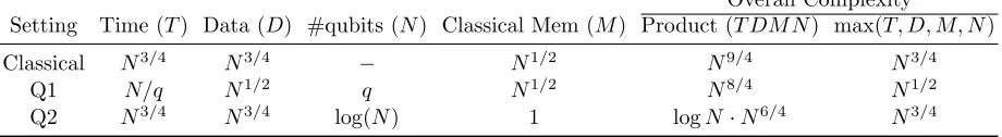
Table 1.Summary of the Attack Complexities against 6-Round Feistel Construction
Overall Complexity
Setting Time (T) Data (D) #qubits (N) Classical Mem (M) Product (T DM N) max(T, D, M, N)
Classical N3/4 N3/4 − N1/2 N9/4 N3/4
Q1 N/q N1/2 q N1/2 N8/4 N1/2
Q2 N3/4 N3/4 log(N) 1 logN·N6/4 N3/4
The range of q in Q1 isq ≤N1/2. All complexities of Q1 are balanced when q =N1/2. Q1 always outperforms classical attacks in terms of the data complexity for any q. Besides, it improves classical attacks in terms of the time complexity whenN1/4≤q≤N1/2.
applying the theory in Sect. 3. Section 5 discusses the attack on Feistel construction when the adversaries can make superposition queries.
2
Preliminaries
This section gives attack models and a summary of the quantum algorithms that are related to our work. Throughout the paper, we assume a basic knowledge of the quantum circuit model. For a public function F : {0,1}n/2 →
{0,1}n/2, we assume that a quantum circuit which calculatesF,C
F :|xi |yi 7→ |xi |y⊕F(x)iis available, andCF runs in a constant time.
2.1 Offline Quantum Computation
If we want to access some data or to operate table look-up in a quantum algorithm without any measurement, we have to set all data on quantum circuits so that data can be accessed in quantum superposition states. In particular, if we want to implement random access to memories, we need as many qubits (or width of the quantum circuit) as the data size. Thus, quantum memory for random access is physically equivalent to quantum processor. We regard that they are essentially identical.
Regardless of whether we use quantum computers or classical computers, the running time of an algorithm significantly depends on how a computational hardware is realized, when the algorithm needs exponentially many hardware resources. Thus if we want to use exponentially many qubits, we have to pay attention to data communi-cation costs in quantum hardwares. In the quantum setting, Bernstein [Ber09] and Banegas and Bernstein [BB17] introduced two communication models, which they call free communication model and realistic communication model. The free communication model assumes that we can operate a unitary operation on any pairs of qubits. On the other hand, the realistic communication model assumes that 2p qubits are arranged as a 2p/2×2p/2 mesh, and a unitary operation can be operated only on a pair of qubits that are within a constant distance. A quantum hardware in the free communication model which hasO(N) qubits can simulate a quantum hardware in the free communication model which hasO(√N) qubits, with time overheadO(√N) [BBG+13].
In this paper, for simplicity, we estimate the time complexity of quantum algorithms in the free communication model. Note that this does not imply that our proposed attacks do not work in the realistic communication model. We design our algorithms so that small quantum processors (of size polynomial in n) parallelly run without any communication between each pair of small processors. Hence if the realistic communication model is applied, time complexity increases by a factor of polynomial inn.
2.2 Related Quantum Algorithms
Problem 2. Suppose a functionφ:{0,1}u→ {0,1}is given as a black box, with a promise that there isxsuch that φ(x) = 1. Then, find xsuch thatφ(x) = 1.
Grover’s algorithm can solve the above problem with O(2u/2) evaluations ofφusing O(u) qubits, ifφ is given as a quantum oracle (or using O(v) qubits, ifφ is given as av-qubit quantum circuit without any measurement). The algorithm is composed of iterations of an elementary step which operatesO(1) evaluation ofφ, and can easily be parallelized [GR04].
If we can use a quantum computer withO(u2p) qubits, we regard it as 2pindependent small quantum processors withO(u) qubits. Then, by parallelly runningO(p2u/2p) iterations on each small quantum processor, we can find xsuch that φ(x) = 1 with high probability. This parallelized algorithm runs in timeO(p2u/2p·T
φ), whereTφ is the time needed to evaluateφonce.
Simon’s Algorithm. Grover’s algorithm is an exponential time algorithm. Here we introduce a quantum algorithm that can solve a problem in polynomial time. The problem is defined as follows:
Problem 3. Letφ:{0,1}u→ {0,1}ube a function such that there is a unique secret valuesthat satisfiesφ(x) =φ(y) if and only ifx=y orx=y⊕s. Then, finds.
Supposeφis given as a quantum oracle. Then, Simon’s algorithm [Sim97] can solve the above problem with O(n) queries, using O(n) qubits. We have to solve a system of linear equations after making queries, which requires O(n3) arithmetic operations. Since any classical algorithm needs exponential time to solve this problem (see the original paper [Sim97] for details), Simon’s algorithm obtains exponential speed-up from classical algorithms. The algorithm can be applied to the problem of which condition “ φ(x) = φ(y) if and only if x= y or x=y⊕s” is replaced with the weaker condition “φ(x⊕s) =φ(x) for any x”, under the assumption thatφsatisfies some good properties [KLLN16a].
Quantum Claw Finding Algorithms. Let us consider two functions f : {0,1}u → {0,1}` and g : {0,1}v →
{0,1}`. If there is a pair (x, y)∈ {0,1}u× {0,1}v such thatf(x) =g(y), then it is called aclaw of the functionsf andg. Now we consider the following problem:
Problem 4. Let u, v be positive integers such that u≥ v. Suppose that two functions f : {0,1}u → {0,1}` and g:{0,1}v→ {0,1}`are given as black boxes. Then, find a claw off andg.
This problem, calledclaw finding problem, has attracted researchers’ attention and is well studied. It is known that, given f and g as quantum oracles, this problem can be solved with O(2(u+v)/3) queries in the case v ≤u < 2v, and O(2u/2) queries in the case 2v ≤ u [BHT97,Amb04,Zha05,Tan09]. Quantum claw finding algorithms and their generalizations already have some applications in attacks against symmetric-key cryptosystems [Kap14,MS17]. Below we assume`=O(u+v).
3
Claw Finding between Classical and Quantum Functions
Quantum claw finding algorithms are useful, though, they cannot be applied if one of target functions, sayg, is not quantum accessible. For example, if we need some information from a classical online (i.e., keyed) oracle to calculate g(y), then we have to use other algorithms, even if we have a quantum computer.
Sections 3 and 4 focus on the Q1 model. Hence, this section considers how to find a claw of functionsf, gwhere gcan be evaluated only classically. We are particularly interested in the case that there exists only a single claw of f andg, and show that the following proposition holds.
Proposition 1. Suppose that f can be implemented on a quantum circuit Cf using O(u+v) qubits, g can be
evaluated only classically, and we can use a quantum computer with O((u+v)2p)qubits. Assume that there exist only a single claw of f andg. Then we can solve Problem 4 in time
OTg,allC + 2u/2+v−(p+pL)/2·TQ f + 2
v−pL+p
, (1)
whereTg,allC is the time to calculate the pair(y, g(y))for ally,TfQ is the time to runCf once, andpL is a parameter
that satisfies pL≤min{p, n}. We also useO(2v)classical memory.
Algorithm. First, evaluateg(y) for all y classically, and store each pair (y, g(y)) in a list L. For eachy ∈ {0,1}v, define a function fy :{0,1}u → {0,1} byfy(x) = 1 if and only if f(x) =g(y). Given Cf and the list L, we can implement fy on a quantum circuit that runs in time O(TfQ) using O(u+v) qubits. Note that the parallelized Grover search onfy, which parallelly runsO(2p−pL) independent small processors, can findx0such thatfy(x0) = 1 (if there exists) in timeO(2u/2−(p−pL)/2·TQ
f ). LetC Grover
y denote this quantum circuit of sizeO((u+v)2p). Then, run the following procedure:
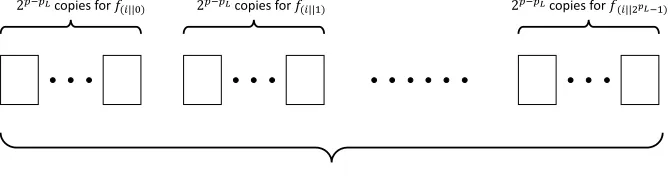
1. For 0≤i≤2v−pL−1, do:
2. RunC(Groverikj) parallelly for 0≤j≤2pL−1 (see Fig. 1).
3. If a pair (x,(ikj)) such thatf(ikj)(x) = 1 is found, then return the pair (x,(ikj)).
In the above procedure, we consider thati, jare elements in{0,1}v−pL and{0,1}pL, respectively, andikj∈ {0,1}v.
2𝑝−𝑝𝐿copies for 𝑓 (𝑖||1)
𝑂 (𝑢 + 𝑣)2𝑝 quantum registers 2𝑝−𝑝𝐿copies for 𝑓
(𝑖||0) 2𝑝−𝑝𝐿copies for 𝑓(𝑖||2𝑝𝐿−1)
Fig. 1.How to useO(2p) qubits
Complexity analysis. To evaluateg(y) and store it for everyy, we needO(Tg,allC ) time andO(2v) classical memory.
In Step 2 of the procedure, the parallelized Grover search on f(ikj) requires time O(2u/2−(p−pL)/2T Q
f ) for each i and j as stated above. In Step 3 of the procedure, we need time O(2p) to check whether a pair (x,(ikj)) such that f(ikj)(x) = 1 exists. Thus, the total running time isO(Tg,allC + 2
v−pL·(2u/2−p/2+pL/2TQ f + 2
p)) = O(TC g,all+ 2u/2+v−p/2−pL/2·TQ
f + 2v−pL +p).
As for the number of qubits, for a fixedi, we useO((u+v)2p−pL) qubits for the parallelized Grover search on f(ikj)for each 0≤j≤2pL−1. Thus the total number of qubits we use isO((u+v)2p−pL)·2pL =O((u+v)2p).
3.1 Variation of Claw Finding
Next, we consider the following variant of the claw finding problem.
Problem 5. Suppose that functionsf :{0,1}u× {0,1}v→ {0,1}`andg:{0,1}v→ {0,1}`are given as black boxes, with promise that there is a unique pair (x, y)∈ {0,1}u× {0,1}v such thatf(x, y) =g(y). Then, find such a pair (x, y).
Again, we assume that g can be evaluated only classically, f can be implemented on a quantum circuit, and ` =O(u+v). Problem 5 appears to be different from Problem 4, however, we can also solve it by applying our algorithm introduced above with a slight modification to the definition offy as:fy(x) = 1 if and only iff(x, y) = g(y). With this small modification, we can find the pair (x, y) such thatf(x, y) =g(y) with the same complexity as in Proposition 1. The next section treats this variant problem to attack Feistel constructions, instead of the original claw finding problem. In what follows, we measurep≤vand 2v≤TC
g,all.
Corollary 1. Suppose thatf can be implemented on a quantum circuitCf usingO(u+v)qubits,gcan be evaluated
only classically, and we can use a quantum computer with O((u+v)2p) qubits, where p≤v. Assume that there is a unique claw off andg. Then we can solve Problem 4 in time
OTg,allC + 2u2+v−p·TQ f
where TC
g,all≥2v is the time to calculate the pair (y, g(y))for all y and T Q
f is the time to runCf once. We also
useO(2v)classical memory.
The algorithms that we introduced in this section assume an ideal situation that we are given a quantum circuit that calculates f without error. However, in real applications, having some error might be inevitable (e.g. we use Grover’s algorithm as a subroutine a few times to calculatef). Nevertheless, if error is small, then the above algo-rithms can still be applied with a small modification. (Roughly speaking, we use quantum amplitude amplification technique [BHMT02] instead of Grover’s algorithm. See Section B in the appendix for details.)
4
Quantum DS-MITM Attacks against Feistel Constructions
In this section, we show that quantum computers can significantly speed-up the DS-MITM attacks even under the limitation that queries are made only in a classical manner (Q1 model). To demonstrate it, we improve on the previous key recovery attack against 6-round Feistel constructions presented by Guo et al. [GJNS14].
4.1 Classical DS-MITM Attack on 6-Round Feistel Constructions
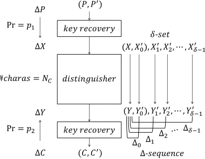
Overview of DS-MITM Attacks We first briefly introduce the framework of the DS-MITM attack. The attack generally consists of the distinguisher and the key-recovery parts as illustrated in Fig. 2. A truncated differential is specified to the entire cipher and suppose that the plaintext difference∆P propagates to the input difference∆X of the distinguisher with probabilityp1. Similarly, the ciphertext difference∆C propagates to the output difference ∆Y of the distinguisher with probability p2 when decryption is performed. The attack is composed of two parts: distinguisher analysis andqueried-data analysis.
𝑘𝑒𝑦 𝑟𝑒𝑐𝑜𝑣𝑒𝑟𝑦
𝑑𝑖𝑠𝑡𝑖𝑛𝑔𝑢𝑖𝑠ℎ𝑒𝑟
𝑘𝑒𝑦 𝑟𝑒𝑐𝑜𝑣𝑒𝑟𝑦 Δ𝑃
Δ𝑋
Δ𝑌
Δ𝐶 Pr = 𝑝1
(𝑋, 𝑋0′), 𝑋
1′, 𝑋2′, ⋯ , 𝑋𝛿−1′
#𝑐ℎ𝑎𝑟𝑎𝑠 = 𝑁𝐶
Pr = 𝑝2
(𝑌, 𝑌0′), 𝑌
1′, 𝑌2′, ⋯ , 𝑌𝛿−1′ 𝛿-𝑠𝑒𝑡
Δ0 Δ1
Δ2 Δ𝛿−1
Δ-𝑠𝑒𝑞𝑢𝑒𝑛𝑐𝑒 (𝑃, 𝑃′)
(𝐶, 𝐶′)
Fig. 2.Overview of DS-MITM Attacks.
In the distinguisher analysis, the attacker enumerates all the possible differential characteristics that can satisfy the specified truncated differential. Suppose that there existNc such characteristics. For each of them, input paired values to the distinguisher are expected to be fixed uniquely. Let (X, X00) be the paired values. Then, the attacker generates a set of texts called δ-set by generating δ−1 new texts Xi0 ← X00 ⊕i for i= 1,2,· · ·, δ−1. Suppose that the corresponding value at the output of the distinguisher can be computed. Let Y, Y00, Y10, Y20,· · ·, Yδ−0 1 be the corresponding values at the output of the distinguisher. The attacker then computes the differences betweenY andYi0 fori= 0,1,· · · , δ−1 and makes a sequence of δoutput differences at the output of the distinguisher. This sequence is called∆-sequence. Note that the difference betweenY andY0
In the queried-data analysis, the attacker makes queries to collect (p1p2)−1 paired values having the plaintext difference ∆P and the ciphertext difference∆C. One pair, with a good probability, satisfies ∆X and ∆Y at the input and output of the distinguisher, respectively. Thus for each of (p1p2)−1 paired values, the attacker guesses subkeys for the key-recovery rounds such that∆X and ∆Y appear after the first and the last key recovery parts, respectively. Then, one of the paired texts (corresponding to P0) is modified toPi0 so that the δ-set is generated at the input to the distinguisher, and those are queried to the oracle to obtain the corresponding ciphertext Ci0. The attacker then processes C0
i with the guessed subkeys for the last key-recovery part, and the ∆-sequence is computed at the output of the distinguisher. Finally, those are matched the list L. If the analyzed pair is a right pair and the guessed subkeys are correct, then a match will be found. Otherwise, a match will not be found as long as (p1p2)−1Nc×2−γδ1.
Application to 6-Round Feistel Constructions. Guo et al. [GJNS14] applied the DS-MITM attack to 6-round Feistel constructions. The attack needs to solve the following problems.
Problem 6. LetF :{0,1}n/27→ {0,1}n/2 be a public function and∆be a fixed difference.
• For a given output difference ∆o, how can we find allv such thatF(v)⊕F(v⊕∆) =∆o?
• For a given input difference∆i, how can we find allv such thatF(v)⊕F(v⊕∆i) =∆?
In the classical attack, those problems can be solved only with 1 access to the precomputed table of size 2n/2. The procedure is rather straightforward. Readers are refer to the paper by Guo et al. [GJNS14] for the exact procedure.
Distinguisher Analysis. The core of the attacks is the 5-round distinguisher explained below. The input and output differences for the 5 rounds are defined as 0kX and Yk0, respectively, whereX, Y ∈ {0,1}n/2, X6=Y. For a given X, Y, the number of the 5-round differential characteristics satisfying those input and output differences is 2n/2. In fact, by representing the n/2-bit difference of the second round-function’s output as Z, the 5-round differential characteristics can be fixed to
(0kX)1stR−→(Xk0)2ndR−→ (ZkX)3rdR−→(YkZ)4thR−→(0kY)5thR−→(Yk0),
which is illustrated in the left-half of Fig. 3.
𝐹
𝐾𝑖
𝐹
𝐾𝑖+1
𝐹
𝐾𝑖+2
𝐹
𝐾𝑖+3
𝐹
𝐾𝑖+4
0 𝑋
𝑌 0
0 0
𝑍 𝑌
𝑋 ⊕ 𝑌 𝑍
𝑍 𝑋
0 𝛿-set
Δ-sequence
𝐹
𝐾0
5𝑅 𝐷𝑖𝑠𝑡𝑖𝑛𝑔𝑢𝑖𝑠ℎ𝑒𝑟
𝑋 ∗
𝑌 0
∗
Δ-sequence
0 𝑋 𝛿-set
0 ∗
𝑝1= 2−𝑛/2
Fig. 3.Left:|Z|Differential Characteristics in the 5-Round Distinguisher. Right: 1-Round Extension for Key-Recovery.
output. Readers are referred to the paper by Guo et al. [GJNS14] for the complete analysis. The computed ∆-sequences are stored in the listL. Note that the size ofδ is very small. Indeed,p1= 2−n/2,p2= 1,Nc= 2n/2 and γ=n/2. Hence,δ= 3 is sufficient to filter out all the wrong candidates.
To balance the complexities between the distinguisher analysis and the queried-data analysis, Guo et al. iterated the above analysis for 2n/4 different choices ofY. More precisely, the n/4 MSBs ofY are always set to 0 andn/4 LSBs ofY are exhaustively analyzed. The complexity of the procedure for each choice ofY isO(2n/2) both in time and memory. Hence, the entire complexity of the distinguisher part isO(23n/4) in both time and memory.
Queried-Data Analysis. Guo et al. appended 1-round before the 5-round distinguisher to achieve the 6-round key-recovery attack, which is illustrated in the right-half of Fig. 3. By propagating the input difference to the distinguisher, 0kX, in backwards,∆P is set toXk∗where∗can be anyn/2-bit difference. The probabilityp1 that a randomly chosen plaintext pair with the differenceXk∗satisfies the difference 0kX after 1 round is 2−n/2.
The attacker collects the pairs that satisfy the truncated differential in Fig. 3 by using the structure tech-nique. Namely, the attacker prepares 2 sets of 2n/2 plaintexts in which the first and the second sets have the form
{(ck0),(ck1),· · ·,(ck2n/2−1)} and {(c⊕Xk0),(c⊕Xk1),· · ·,(c⊕Xk2n/2−1)}, respectively, where c is a ran-domly chosenn/2-bit constant. About 2n pairs exist whereas only O(2n/4) pairs satisfy∆C in the corresponding ciphertexts. By iterating this procedureO(2n/4) times for different choices ofc, the attacker collectsO(2n/2) pairs satisfying the truncated differential in Fig. 3. In summary, withO(23n/4) queries (and thus the time complexity of O(23n/4) memory accesses),O(2n/2) pairs are obtained, in which one pair will satisfy the probabilistic differential propagation in the first round.
For each pair, the input and output differences ofF in the first round are fixed, which will fixK0uniquely. The attacker then modifies the left-half of the plaintext such thatδ-set withδ= 3 is generated at the right-half of the input to the distinguisher. The right-half of the plaintext is also modified to ensure that the left-half of the input to the distinguisher is not affected. The modified plaintexts are then queried to obtain the corresponding ciphertexts. The attacker computes the corresponding∆-sequence and matches L; the list computed during the distinguisher analysis. A match recoversK0andZ. The other subkeys are trivially recovered from the second round one by one.
Summary of Complexity. In the distinguisher analysis, both of the time and memory complexities are O(23n/4). In the queried-data analysis, the data and time complexities areO(23n/4) and it uses a memory of size O(2n/2) to collect the pairs with the structure technique.
Remarks. Solving Problem 6 is rather straightforward in the classical attack with O(2n/2) memory, whereas this is a crucial problem to the quantum adversaries. This is because the efficient table look-up cannot be executed in quantum computers.
4.2 Quantum DS-MITM Attack on 6-Round Feistel Constructions
We now convert the classical DS-MITM attack on 6-round Feistel constructions into quantum one, in which the adversary has access to a quantum computer to perform offline computations whereas queries are made in the classical manner. The attack complexity becomesO(2n/2) queries,O(2n/2) offline quantum computations by using O(2n/2) qubits.
The main idea is to introduce quantum operations to reduce the complexity of the distinguisher analysis. We show that the claw finding algorithm in Sect. 3 can be used to find a match between the distinguisher and the queried-data analyses. This enables us to adjust the tradeoff between the complexities in the distinguisher and the queried-data analyses, and thus the data complexity can also be reduced.
Switching Online and Offline Phases. The claw finding algorithm in Sect. 3 matches the result of the quantum computation against the results collected in the classical method. Namely, the results of the queried-data analysis must be stored before the distinguisher analysis starts.
This can be easily done by switching the order of the two analyses. In fact, such a switch has already been applied by Darbez and Perrin [DP15, Appendix E] though their goal is to optimize the classical attack complexity, which is different from ours.
Queried-Data Analysis. Because queries are made in the classical manner, the procedure of the queried-data analysis remains unchanged from the classical attack by Guo et al. However, to directly apply the claw finding algorithm to the DS-MITM attack, we explicitly separate the procedure to collectp−11 = 2n/2 pairs satisfying the truncated differentials (both∆P and∆C) and the procedure to compute∆-sequences.
Precomputation for Collecting Pairs. The goal of this procedure is to collect 2n/2 pairs satisfying both∆P =Xk∗ and∆C=∗k0. To use the structure technique, we query 2 sets of 2n/2plaintexts{(ck0),(ck1),· · ·,(ck2n/2−1)}and
{(c⊕Xk0),(c⊕Xk1),· · ·,(c⊕Xk2n/2−1)}. About 2n pairs can be generated and 2n/2of them have no difference in the right-half of the ciphertexts. The generated pairs are stored in the listLpreindexed by the differenceY (the left-half of∆C). In summary, this procedure requiresO(2n/2) classical queries,O(2n/2) memory access andO(2n/2) classical memory.
Generating∆-sequences. The goal of this procedure is to generate∆-sequences for all the pairs stored inLpre. To make it consistent with the notations in Sect. 3, we define a classical functiong:{0,1}n/2→ {0,1}δn/2 that takes the differenceY (the left-half of∆C) as input and outputs the∆-sequence as follows.
1. Pick up all the pairs inLpre such that the differenceY matches theg’s input.
2. Compute the∆-sequences as in the classical attack by assuming that the probabilistic differential propagation in the first round is satisfied.
Then, the classical queried-data analysis becomes identical with computingg(y) for ally∈Y. The cost of computing gfor a single choice of yis 1. Hence, with the notation in Sect. 3,Tg,allC becomes O(2n/2). After this phase, a listL with a classical memory that storesO(2n/2)∆-sequences is generated.
Quantum Distinguisher Analysis. The goal of the distinguisher analysis is to calculate ∆-sequences for all 2n/2 choices ofY and 2n/2 choices ofZ in Fig. 3 in order to find a match withL. We define a quantum function f : {0,1}n/2× {0,1}n/2 → {0,1}δn/2 that takes Z and Y as input and calculates the corresponding∆-sequence. Given that L is computed before this analysis, the goal can be viewed as searching for a preimage Z such that
∃Y, f(Z, Y)∈L.
An Issue to be taken into account. Note that in our situation, the function f might be incompletely defined. We want to define f(Z, Y) to be the corresponding ∆-sequence to (Z, Y), however, to be precise, we will have the following issue when Problem 6 is solved.
Issue. To calculate the corresponding ∆-sequence, we need input/output pairs of the 2nd, 3rd, and 4th round functions that are compatible with the pair (Z, Y). Though there exists one suitable pair for each round function on average, there might be no pair or more than one pair that are compatible with the pair (Z, Y).
This issue already exists even in the classical setting, but it is trivially solved. However, solving the issue in the quantum setting is non-trivial, and deserves careful attention. In what follows, for simplicity, we first describe the attack by assuming that the above issue is naturally solved as in the classical setting, and later explain how to deal with it.
Quantum procedures and complexity. Assume thatf(Z, Y) is uniquely determined for each (Z, Y). Remember that the goal of the quantum distinguisher analysis is to findZ such that∃Y, f(Z, Y)∈L. As discussed in Corollary 1, suppose that a quantum circuit Cf that calculatesf(Z, Y) for a single choice of (Z, Y) in timeTfQ can be imple-mented by usingO(n) qubits and we can use a quantum computer with O(n2p) qubits. Then the time complexity to find suchZ becomes O(2n/4+n/2−p·TQ
f + 2 n/2).
1. Find the input/output pair of the 2nd round functionF that has input differenceX and output differenceZ. 2. Find the input/output pair of the 3rd round functionF that has input differenceZ and output differenceX⊕Y. 3. Find the input/output pair of the 4th round function F that has input differenceY and output differenceZ. 4. Construct a δ-set and calculate the corresponding∆-sequence, using the result of Steps 1, 2, and 3.
5. Output the∆-sequence obtained in Step 4.
Steps 1,2, and 3 correspond to Problem 6, which was solved using an efficient table look-up in the classical setting. However, in our circuitCf, we use the Grover search to find the input/output pairs, since there is an obstacle that quantum computer cannot perform an efficient table look-up. Because the input and output sizes of F are n/2 bits, we can run Steps 1,2, and 3 with Grover’s algorithm in timeO(2n/4), usingO(n) qubits. The complexities of Steps 4 and 5 are much smaller than that of the application of Grover’s algorithm. Hence the above Cf runs in timeTfQ =O(2n/4), usingO(n) qubits. Note thatCf may return an error with a small probability since we use the Grover search as subroutines for a few times. However we can deal with this error, as explained in Sect. 3.
As described in Corollary 1, if O(n2p) qubits are available (p≤n/2), then we can find Zsuch thatf(Z, Y)∈L in time O(2n/4+n/2−p+n/4+ 2n/2) =O(2n−p). Complexities are balanced at p=n/2. In summary, we can find a match with time complexityO(2n/2), usingO(n2n/2) qubits.
Dealing with the issue. Next, we explain how to deal with the issue described above. We regard that each element in{0,1}n/2is a binary representation of an integer i(0≤i≤2n/2−1).
As described before, to calculate the value f(Z, Y), we have to calculate input and output pairs of the 2nd, 3rd, and 4th round functions that are compatible withZ, Y (andX). More concretely, we have to calculate a tuple (α2, α3, α4) that satisfiesF(α2)⊕F(α2⊕X) =Z(the condition for the 2nd round function), andF(α3)⊕F(α3⊕Z) = X⊕Y (the condition for the 3rd round function), andF(α4)⊕F(α4⊕Y) =Z (the condition for the 4th round function). Without loss of generality, we assumeα2< α2⊕X, α3< α3⊕Z, α4< α4⊕Y. Remember that the issue is that there might be no such tuple (α2, α3, α4), or more than one tuples that are compatible withZ, Y.
If there is no tuple that is compatible with (Z, Y), we simply putf(Z, Y) :=⊥. The problem is that there might be more than one tuples that are compatible with (Z, Y). In the classical setting, the number of solutions for a given (Z, Y) can be obtained easily by looking-up a precomputation table. On the other hand, in the quantum setting, we need to iterate Grover’s algorithm multiple times if there are more than one tuples, thus the complexity of this part increases as proportional to the number of tuples.
Now we assume that the following property holds: for arbitrary d6=d0 ∈ {0,1}n/2\ {0n/2}, there are at most Nmax := d3(n2 −1)/log(n2 −1)emany bit-strings αthat satisfies F(α)⊕F(α⊕d) = d0 and α < α⊕d. This is a reasonable assumption since, for a random function φ: {0,1}u → {0,1}u, we have Pr[|φ−1(d0)| ≤3u/logu] ≥ 1−1/2u (see Lemma 5.1 in [MU05]), andF(·)⊕F(· ⊕d) is an almost random function if F is random (and here we consider that the domain ofF(·)⊕F(· ⊕d) is{x|x < x⊕d}, of which cardinality is 2n/2−1).
To avoid the problem that there might be more than one tuples, we divide the problem intoN3
max cases, and associate a triplet (i, j, k) with each case (0≤i, j, k≤Nmax−1). We run the quantum distinguish analysis described above for each cases, i.e., run it N3
max times. In the case (i, j, k), we search for α2, α3, α4 from the sets of strings of which most significant logNmax bits arei, j, andk, respectively. By our assumption described above, there is at most only one tuple (α2, α3, α4) in each case, and the problem does not occur in each case.
Trying allNmax3 cases increases the time complexity by a factor ofNmax3 . However, we run the Grover search on the restricted domains for each case, and thus the time complexity decreases by a factor of√Nmax. Consequently, dealing with the issue increases the time complexity by a factor ofNmax3 /√Nmax=N
5/2
max=O(n5/2).
Complexity Summary. The complexity of the attack is as follows.
• The queried-data analysis requiresO(2n/2) classical queries,O(2n/2) computations andO(2n/2) classical mem-ory.
• The quantum distinguisher analysis requires O(n2n/2) qubits andO(n5/22n/2) offline computations.
5
Attacks Using Quantum Queries
This section discusses quantum attacks in the Q2 model. That is, an adversary is allowed to make quantum superposition queries to online oracles. We show that we can recover full keys of anr-round Feistel construction (r > 3) in time O(n32n(r−3)/4), using O(n2) qubits. Our idea is to combine the trivial key-recovery attack using Grover search with the quantum distinguisher of 3-round Feistel construction by Kuwakado and Morii [KM10], which was later generalized by Kaplan et al. [KLLN16a]. To combine them, we apply the technique by Leander and May [LM17], with a little adjustment. We also show in Sect. 5.2 how to simulate the “half output oracle” given a usual complete encryption oracle, which solves the controversial issue in the quantum distinguisher by Kuwakado and Morii (see Problem 1).
Again, we considern-bit Feistel constructions such that eachn/2-bit round key is added before round function F. We do not consider parallelization for quantum query attacks, since it seems unreasonable to assume that there are many copies of the online oracle and an adversary is allowed to parallelly access to them.
5.1 Quantum Distinguisher of 3-Round Feistel Constructions
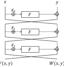
We briefly explain the quantum attack that distinguishes 3-round Feistel constructions from a random permutation π[KM10,KLLN16a]. The attack works in the Q2 model, and runs in polynomial time due to Simon’s algorithm.
Assume that we are given a quantum oracle that calculatesW(x, y), the rightn/2-bits of the ciphertext which is encrypted with 3-round Feistel constructions (see Fig. 5.1). Then,W(x, y) =x⊕F(K1⊕y⊕F(K0⊕x)) holds. Now,
𝐹
𝐾0
𝐹
𝐾1
𝐹
𝐾2
𝑥 𝑦
𝑊(𝑥, 𝑦) 𝑉(𝑥, 𝑦)
Fig. 4.3-round Feistel constructions
fix two different bit strings α, β ∈ {0,1}n/2 and definef : {0,1}n/2+1 → {0,1}n/2 byf(0, x) :=W(α, x)⊕β and f(1, x) :=W(β, x)⊕αforx∈ {0,1}n/2. Then simple calculation shows thatf((b, x)⊕(1, F(K
0⊕α)⊕F(K0⊕β))) =f(b, x) holds, i.e.,f has a period (1, F(K0⊕α)⊕F(K0⊕β)).
On the other hand, if we are given a quantum oracle that calculates the right n/2-bits of π(x, y) instead of W(x, y), and construct such a functionf, thenf does not have such a period with high probability. Thus, roughly speaking, we can distinguish 3-round Feistel constructions from a random permutationπwith high probability by using Simon’s algorithm.
5.2 Truncating Outputs of Quantum Oracles
Let O :|xi |yi |zi |wi 7→ |xi |yi |z⊕OL(x, y)i |w⊕OR(x, y)ibe the complete encryption oracle, where OL, OR denote the left and right n/2-bits of the complete encryption, respectively. Our goal is to simulate oracle OR :
|xi |yi |wi 7→ |xi |yi |w⊕OR(x, y)i. Instead of simulating OR itself, it suffices to simulate an operator O0R :
|xi |yi |wi |0n/2i 7→ |xi |yi |w⊕OR(x, y)i |0n/2i using ancilla qubits. Let |+i := Hn/2|0n/2i, where Hn/2 is an n/2-bit Hadamard gate. ThenO |xi |yi |+i |wi=|xi |yi |+i |w⊕OR(x, y)iholds for anyx, y, w∈ {0,1}n/2.
Now, defineO0
R:= (I⊗Hn/2)·Swap· O ·Swap·(I⊗Hn/2), whereSwapis an operator that swaps lastn-qubits:
|xi |yi |zi |wi 7→ |xi |yi |wi |zi. Then easy calculations show thatO0
R|xi |yi |wi |0n/2i=|xi |yi |w⊕OR(x, y)i |0n/2i holds. Hence we can simulateOR given the complete encryption oracle O, using ancilla qubits.
5.3 Grover Meets Simon Technique and Adjustment for Feistel Constructions
To combine the quantum distinguisher described above with key recovery using the Grover’s search, we use a technique by Leander and May [LM17]. They proposed the technique that combines Grover’s algorithm with Simon’s algorithm, to recover keys of FX constructions.
We want to apply it to Feistel constructions, however, some adjustment is needed since their algorithm is dedicatedly designed to attack FX constructions. In this section, we first describe the original proposition by Leander and May, then describe our adjusted proposition, and finally describe difference between them.
The original technique. The following proposition is the original technique by Leander and May [LM17].
Proposition 2 (Theorem 2 in [LM17]). Let Ψ :Fm
2 ×Fn2 →Fn2 be a function such that Ψ(k,·) :Fn2 →Fn2 is a random function for any fixedk∈Fn
2. SupposeΨ is public, and an adversary can calculate it offline. Fork0∈ {0,1}m and k1, k2 ∈ {0,1}n, let Φ
k0,k1,k2 : F m
2 ×F32n → Fn2 be the function defined by Φk0,k1,k2(x) = Ψ(k0, x⊕k1)⊕k2. Then, given quantum oracle accesses to Φk0,k1,k2(·), we can recover (k0, k1, k2) with a constant probability and O((m+n)2m/2)queries, usingO(m+n2)qubits.
Leander and May’s algorithm firstly defines functionΦ0:Fm2 ×F n 2 →F
n
2 byΦ0(k, x) =Φk0,k1,k2(x)⊕Ψ(k, x). Since Φ0(k0, x⊕k1) =Ψ(k0, x⊕k1)⊕k2⊕Ψ(k, x) =Φ0(k0, x) holds,Φ0(k0,·) has a periodk1. Roughly speaking, their algorithm searches for the correct keyk0with the Grover search, and checks whether or not each candidate keykis correct by checking whetherΦ0(k,·) is periodic or not, by running many independent Simon’s algorithm parallelly. The Grover search for anm-bit keyk0requiresO(m) qubits.O(n) parallel Simon’s algorithm requiresO(n2) qubits. Thus the above algorithm needsO(m+n2) qubits.
Note that the above proposition refers only to query complexity, but not to time complexity. In the above algorithm,O(n3) arithmetic are needed to solve linear equations afterO(n) queries are made by Simon’s algorithm (see Section 2.2). This is the essential point that makes difference between the query complexity and the time complexity. Taking theseO(n3) operations into account, the running time of their algorithm isO((m+n3)2m/2).
Adjusted technique. Now we describe our adjusted technique, which can be proven in the similar way as the original proposition. In the next section,k0 in Proposition 3 will correspond to subkeys of the last (r−3)-rounds K3, . . . , Kr−1ofr-round Feistel constructions, andk1 will correspond to the hidden period in the quantum distin-guishing attack introduced in Section 5.1.
Proposition 3. Let Ψ :Fm2 ×Fn2 → F2n be a function such that Ψ(k,·) : Fn2 →Fn2 is a random function for any fixed k∈Fn2. Let Φ:Fm2 ×Fn2 →Fn2 be a function such that Φ(k,·) :Fn2 →Fn2 is a random function for any fixed k ∈ Fn2 \ {k0}, and Φ(k0, x) = Ψ(k0, x⊕k1). Then, given quantum oracle accesses to Φ(·,·) and Ψ(·,·), we can recover (k0, k1)with a constant probability andO((m+n2)2m/2)queries, usingO(m+n2) qubits.
The difference between Proposition 2 and Proposition 3. Here we explain how our algorithm (and our problem that it solves) in Proposition 3 differs from the original algorithm (Proposition 2).
In the original problem (Proposition 2),Ψ is assumed to be a public function (that is, adversary can calculateΦ offline), andΦk0,k1,k2 is given as an online oracle. On the other hand, in our problem (Proposition 3), both of two functionsΦandΨ are given as online oracles, and adversary cannot calculate them offline. In addition, the domain size ofΦk0,k1,k2 in the original problem differs from that ofΦin our problem. These lead to the difference of query complexities between the original proposition and ours. See Appendix C for details.
In the situation that we want to combine Grover’s and Simon’s algorithm and we are given two keyed quantum oracles, the original proposition cannot be applied and some modification such as Proposition 3 is required.
5.4 Combining the Quantum Distinguisher with Key Recovery Attacks
This section explains how to apply Proposition 3 to extend the quantum distinguisher in Section 5.1 to key recovery attacks. We begin with explaining intuition behind our attack.
Consider to guess subkeys for the last (r−3)-roundsK3, . . . , Kr−1, given the quantum encryption oracle of an r-round Feistel construction. Let us suppose the guess is correct. Then we can implement a quantum circuit that calculates the first three rounds of the Feistel construction. On the other hand, if the guess is incorrect, then the corresponding quantum circuit will be the circuit that calculates an almost random function. Hence we can check the correctness of the guess by using the 3-round quantum distinguisher. We guessK3, . . . , Kr−1by using Grover’s algorithm, while we use Simon’s algorithm for the 3-round distinguisher.
Next, we describe details of our attack. Assume that we are given the quantum encryption oracle of an r-round Feistel construction Encr : {0,1}n → {0,1}n. For k = (K0
3, . . . , Kr−0 1)∈ {0,1}(r−3)n/2, let Dk : {0,1}n →
{0,1}n denote the partial decryption of the last (r−3)-rounds with the key candidate (K0
3, . . . , Kr−0 1). Define W :{0,1}(r−3)n/2× {0,1}n/2× {0,1}n/2→ {0,1}n/2 be the function defined by
W(k, x, y) := the right halfn/2-bits ofDk◦Encr(x, y). (3)
We can implement a quantum circuit of W using the quantum oracle of Encr and the simulating technique we described in Section 5.2. Note thatW(k0, x, y) =x⊕F(K1⊕y⊕F(K0⊕x)) holds, wherek0= (K3, . . . , Kr−1) is the set of correct partial keys of the Feistel constructionEncrfrom the 4-th round to the last round.
Now, fix two different n/2-bit stringsα, β, and defineΨ, Φ:{0,1}(r−3)n/2× {0,1}n/2→ {0,1}n/2 byΨ(k, x) := W(k, α, x)⊕β and Φ(k, x) := W(k, β, x)⊕α. Then Ψ(k,·) is an almost random function for each k, and Φ(k,·) is also an almost random function for each k 6= k0. In addition, Φ(k0, x) = Ψ(K0, x⊕k1) holds, where k1 = F(α⊕K0)⊕F(β⊕K0), since
Φ(k0, x) =W(k0, β, x)⊕α=β⊕F(K1⊕x⊕F(β⊕K0))α
=α⊕F(K1⊕x⊕F(β⊕K0)⊕F(α⊕K0)⊕F(α⊕K0))⊕β=W(k0, α, x⊕k1)⊕β=Ψ(k0, x⊕k1).
Thus, by applying Proposition 3, we can recover the round keysK3, . . . , Kr−1. After we obtainK3, . . . , Kr−1, we can construct a quantum circuit that calculates the first 3 rounds of the Feistel construction. Hence, for arbitrary α, β∈ {0,1}n/2such thatα=6 β, we can computeF(α⊕K0)⊕F(β⊕K0) in polynomial time by using the 3-round distinguisher. Then we can recover K0 in time O(2n/4) by using the Grover search. Once K0, K3, . . . , K
r−1 are recovered, we can easily recoverK1, K2in time O(2n/4) by using the Grover search.
Complexity. Consequently, we can recoverK0, . . . Kr−1in timeO(n32(r−3)n/4), usingO(n2) qubits. In particular, for the caser= 6, all the complexities are balanced at ˜O(2n/2), which is the same as the attack in Section 4:
• The attack requiresO((m+n2)2n) queries,O(n32n/2) computations, andO(m+n2) qubits. No classical memory is required in this attack.
References
AC18. Carlisle Adams and Jan Camenisch, editors. Selected Areas in Cryptography - SAC 2017 - 24th International
Conference, Ottawa, ON, Canada, August 16-18, 2017, Revised Selected Papers, volume 10719 ofLecture Notes
in Computer Science. Springer, 2018.
Amb04. Andris Ambainis. Quantum walk algorithm for element distinctness. In 45th Symposium on Foundations of
Computer Science (FOCS 2004), 17-19 October 2004, Rome, Italy, Proceedings, pages 22–31. IEEE Computer
Society, 2004.
BB17. Gustavo Banegas and Daniel J. Bernstein. Low-communication parallel quantum multi-target preimage search. In Adams and Camenisch [AC18], pages 325–335.
BBG+13. Robert Beals, Stephen Brierley, Oliver Gray, Aram W Harrow, Samuel Kutin, Noah Linden, Dan Shepherd, and
Mark Stather. Efficient distributed quantum computing. Proc. R. Soc. A, 469(2153):20120686, 2013.
BBHT98. Michel Boyer, Gilles Brassard, Peter Høyer, and Alain Tapp. Tight bounds on quantum searching. Fortschritte
der Physik, 46(4-5):493–505, 1998.
Ber09. Daniel J Bernstein. Cost analysis of hash collisions: Will quantum computers make sharcs obsolete?SHARCS’09
Special-purpose Hardware for Attacking Cryptographic Systems, page 105, 2009.
BHMT02. Gilles Brassard, Peter Høyer, Michele Mosca, and Alain Tapp. Quantum amplitude amplification and estimation.
Contemporary Mathematics, 305:53–74, 2002.
BHT97. Gilles Brassard, Peter Høyer, and Alain Tapp. Quantum cryptanalysis of hash and claw-free functions. SIGACT News, 28(2):14–19, 1997.
Bon17. Xavier Bonnetain. Quantum key-recovery on full AEZ. In Adams and Camenisch [AC18], pages 394–406. DDKS15. Itai Dinur, Orr Dunkelman, Nathan Keller, and Adi Shamir. New attacks on Feistel structures with improved
memory complexities. In Rosario Gennaro and Matthew Robshaw, editors,Advances in Cryptology - CRYPTO
2015 - 35th Annual Cryptology Conference, Santa Barbara, CA, USA, August 16-20, 2015, Proceedings, Part I,
volume 9215 ofLecture Notes in Computer Science, pages 433–454. Springer, 2015.
DFJ13. Patrick Derbez, Pierre-Alain Fouque, and J´er´emy Jean. Improved key recovery attacks on reduced-round AES in the single-key setting. In Thomas Johansson and Phong Q. Nguyen, editors, Advances in Cryptology - EU-ROCRYPT 2013, 32nd Annual International Conference on the Theory and Applications of Cryptographic
Tech-niques, Athens, Greece, May 26-30, 2013. Proceedings, volume 7881 ofLecture Notes in Computer Science, pages
371–387. Springer, 2013.
DP15. Patrick Derbez and L´eo Perrin. Meet-in-the-middle attacks and structural analysis of round-reduced PRINCE. In Gregor Leander, editor,Fast Software Encryption - 22nd International Workshop, FSE 2015, Istanbul, Turkey,
March 8-11, 2015, Revised Selected Papers, volume 9054 ofLecture Notes in Computer Science, pages 190–216.
Springer, 2015.
DS08. H¨useyin Demirci and Ali Aydin Sel¸cuk. A meet-in-the-middle attack on 8-round AES. In Kaisa Nyberg, editor,
Fast Software Encryption, 15th International Workshop, FSE 2008, Lausanne, Switzerland, February 10-13, 2008,
Revised Selected Papers, volume 5086 ofLecture Notes in Computer Science, pages 116–126. Springer, 2008.
DW17. Xiaoyang Dong and Xiaoyun Wang. Quantum key-recovery attack on Feistel structures.IACR Cryptology ePrint
Archive, 2017:1199, 2017.
GJNS14. Jian Guo, J´er´emy Jean, Ivica Nikolic, and Yu Sasaki. Meet-in-the-middle attacks on generic Feistel constructions. In Palash Sarkar and Tetsu Iwata, editors, Advances in Cryptology - ASIACRYPT 2014 - 20th International Conference on the Theory and Application of Cryptology and Information Security, Kaoshiung, Taiwan, R.O.C.,
December 7-11, 2014. Proceedings, Part I, volume 8873 ofLecture Notes in Computer Science, pages 458–477.
Springer, 2014.
GJNS16. Jian Guo, J´er´emy Jean, Ivica Nikolic, and Yu Sasaki. Meet-in-the-middle attacks on classes of contracting and expanding Feistel constructions. IACR Trans. Symmetric Cryptol., 2016(2):307–337, 2016.
GR04. Lov K. Grover and Terry Rudolph. How significant are the known collision and element distinctness quantum algorithms? Quantum Information & Computation, 4(3):201–206, 2004.
Gro96. Lov K. Grover. A fast quantum mechanical algorithm for database search. In Gary L. Miller, editor,Proceedings of the Twenty-Eighth Annual ACM Symposium on the Theory of Computing, Philadelphia, Pennsylvania, USA,
May 22-24, 1996, pages 212–219. ACM, 1996.
HS18. Akinori Hosoyamada and Yu Sasaki. Cryptanalysis against symmetric-key schemes with online classical queries and offline quantum computations. InTopics in Cryptology - CT-RSA 2018 - The Cryptographers’ Track at the
RSA Conference 2018, San Francisco, CA, USA, April 16-20, 2018, Proceedings, pages 198–218, 2018.
IS12. Takanori Isobe and Kyoji Shibutani. All subkeys recovery attack on block ciphers: Extending meet-in-the-middle approach. In Lars R. Knudsen and Huapeng Wu, editors, Selected Areas in Cryptography, 19th International
Conference, SAC 2012, Windsor, ON, Canada, August 15-16, 2012, Revised Selected Papers, volume 7707 of
IS13. Takanori Isobe and Kyoji Shibutani. Generic key recovery attack on Feistel scheme. In Kazue Sako and Palash Sarkar, editors,Advances in Cryptology - ASIACRYPT 2013 - 19th International Conference on the Theory and
Application of Cryptology and Information Security, Bengaluru, India, December 1-5, 2013, Proceedings, Part I,
volume 8269 ofLecture Notes in Computer Science, pages 464–485. Springer, 2013.
Kap14. Marc Kaplan. Quantum attacks against iterated block ciphers. CoRR, abs/1410.1434, 2014.
KLLN16a. Marc Kaplan, Ga¨etan Leurent, Anthony Leverrier, and Mar´ıa Naya-Plasencia. Breaking symmetric cryptosystems using quantum period finding. In Matthew Robshaw and Jonathan Katz, editors, Advances in Cryptology -CRYPTO 2016 - 36th Annual International Cryptology Conference, Santa Barbara, CA, USA, August 14-18,
2016, Proceedings, Part II, volume 9815 ofLecture Notes in Computer Science, pages 207–237. Springer, 2016.
KLLN16b. Marc Kaplan, Ga¨etan Leurent, Anthony Leverrier, and Mar´ıa Naya-Plasencia. Quantum differential and linear cryptanalysis. IACR Trans. Symmetric Cryptol., 2016(1):71–94, 2016.
KM10. Hidenori Kuwakado and Masakatu Morii. Quantum distinguisher between the 3-round Feistel cipher and the random permutation. InIEEE International Symposium on Information Theory, ISIT 2010, June 13-18, 2010,
Austin, Texas, USA, Proceedings, pages 2682–2685. IEEE, 2010.
KM12. Hidenori Kuwakado and Masakatu Morii. Security on the quantum-type Even-Mansour cipher. InProceedings of the International Symposium on Information Theory and its Applications, ISITA 2012, Honolulu, HI, USA,
October 28-31, 2012, pages 312–316. IEEE, 2012.
Knu02. Lars R. Knudsen. The security of Feistel ciphers with six rounds or less. J. Cryptology, 15(3):207–222, 2002. LM17. Gregor Leander and Alexander May. Grover meets Simon - quantumly attacking the FX-construction. In Tsuyoshi
Takagi and Thomas Peyrin, editors,Advances in Cryptology - ASIACRYPT 2017 - 23rd International Conference on the Theory and Applications of Cryptology and Information Security, Hong Kong, China, December 3-7, 2017,
Proceedings, Part II, volume 10625 ofLecture Notes in Computer Science, pages 161–178. Springer, 2017.
MBTM17. Kerry A. McKay, Larry Bassham, Meltem Snmez Turan, and Nicky Mouha. NISTIR 8114 Report on Lightweight Cryptography. Technical report, U.S. Department of Commerce, National Institute of Standards and Technology, 2017.
MS17. Bart Mennink and Alan Szepieniec. XOR of PRPs in a quantum world. In Tanja Lange and Tsuyoshi Takagi, editors,Post-Quantum Cryptography - 8th International Workshop, PQCrypto 2017, Utrecht, The Netherlands,
June 26-28, 2017, Proceedings, volume 10346 of Lecture Notes in Computer Science, pages 367–383. Springer,
2017.
MU05. Michael Mitzenmacher and Eli Upfal. Probability and Computing: Randomized Algorithms and Probabilistic
Analysis. Cambridge University Press, 2005.
Sim97. Daniel R. Simon. On the power of quantum computation. SIAM J. Comput., 26(5):1474–1483, 1997. Tan09. Seiichiro Tani. Claw finding algorithms using quantum walk. Theor. Comput. Sci., 410(50):5285–5297, 2009. Zha05. Shengyu Zhang. Promised and distributed quantum search. In Lusheng Wang, editor,Computing and
Combina-torics, 11th Annual International Conference, COCOON 2005, Kunming, China, August 16-29, 2005, Proceed-ings, volume 3595 ofLecture Notes in Computer Science, pages 430–439. Springer, 2005.
A
On Quantum Amplitude Amplification
This section briefly explains thequantum amplitude amplificationtechnique, which is developed by Brassard, Høyer, Mosca, Tapp [BHMT02] since the later sections in the appendix need it.
Proposition 4 (Quantum Amplitude Amplification [BHMT02]).LetAbe a quantum algorithm onuqubits without any measurement. Let B:{0,1}u→ {0,1} be a boolean function. We call an element x∈ {0,1}u is good
if B(x) = 1, and badotherwise. Define unitary operators SB andS0 on u-qubit states by
SB:|xi 7→
(
− |xi if xis good,
|xi otherwise, (4)
and
S0:|xi 7→
(
− |xi if x= 0,
|xi otherwise. (5)
Let abe the probability that we obtain a good element xwhen we measureA |0i. DefineQ:=−AS0A−1SB and let t >0be an integer. Then, the probability that we obtain a goodxwhen we measureQtA |0iis equal tosin2((2t+1)θ
a),
We need this proposition in the appendix C. Below we call B classifier, following the work by Leander and May [LM17]. Note that, if there is a O(u)-qubit quantum circuit that calculates B in time TB, thenSB can be implemented on a quantum circuit with O(u)-qubits so that it runs in time O(TB). In the above proposition, we have to know or estimate the probabilityabefore running algorithms, which may not be possible in some situations. However, actually we can find a good element even if we do not know the probabilityain advance.
Proposition 5 (Quantum Amplitude Amplification, without knowinga [BHMT02]). Let abe the prob-ability that we obtain a good element xwhen we measure A |0i. Then, there is a quantum algorithm that runs in timeO(p1/a(TA+TB))that finds a good elementxwith constant probability. Here, TA andTB are the time that
is required to run Aand evaluateB on a quantum circuit, respectively.
The algorithm in Proposition 5 is described as the following procedures. First, a sequence of positive integers t1, t2, . . . is defined. Second, the algorithm run the following procedure for eachi≥1: run the quantum circuitQtiA on the initial state|0i, and measure the final quantum state. If a good elementxis obtained, then the algorithm outputsxas a result, and stops. If the algorithm cannot find such a good element, then it runs forever.
If A is an Hadamard gate, quantum amplitude amplification matches the Grover search on B, and thus this technique is a generalization of the Grover search. In the similar way as for the Grover search, quantum amplitude amplification can be parallelized. If O(u2p) qubits are available, then we regard them as O(2p) small quantum processors of size O(u). By running the algorithm on those small processors, we can find a good element in time O(p1/a2p(T
A+TB)).
B
Dealing with Small Errors of
f
This section shows that Corollary 1 is still valid even if f can be calculated only with some small error. We use the quantum amplitude amplification technique (see Appendix C) instead of the Grover search. Suppose that our goal is to find xsuch thatf(x, y0) =g(y0) for a fixedy0 ∈ {0,1}v. Assume w, `=O(u+v), and we only have a quantum circuitCf0 that calculatesf with some error:
Cf0 :|xi |y0i |0 w+`
i 7→q1−δ2
x,y0|xi |y0i |ψx,y0i |f(x, y0)i+δx,y0|xi |y0i |garbagei,
for somew-qubit state|ψx,y0i, which contains some necessary intermediate information to calculatef(x, y0), and (w+`)-qubit state|garbagei, which corresponds to unnecessary information. Here we assume thatf is calculated by using the Grover search that normally contains some small error, and we now assume that δx,y0 =O(1/2
u/2).
LetU⊕y0 denote the unitary operator|zi 7→ |z⊕y0i. With the notations in Proposition 4, we put A:=C 0 f·(H
u⊗
U⊕y0⊗Iw+`), which suggests that
A |0u+v+w+`i=Cf0 p1/2uX x
|xi |y0i |0w+`i
!
=p1/2uX x
q
1−δ2
x,y0|xi |y0i |ψx,y0i |f(x, y0)i+δx,y0|xi |y0i |garbagei
,
where Hu is the Hadamard operator of dimension on u-qubit states andI
w+` is the identity operator on (w+ `)-qubit states. Now we run the quantum amplitude amplification with the aboveA, defining that the “good” element corresponds to a state such that the last `-qubits match g(y0). That is, we define B: {0,1}u+v+w+` → {0,1} by
B(α) = 1 if and only if the last`-bits ofαisg(y0). A quantum circuit ofBcan be implemented usingO(u+v)-qubits since we already know (y0, g(y0)). Then, the good probability is roughly equals to 1/2u, which suggests that we can find xsuch that fy0(x) = 1 in time O(2
u/2). Thus our algorithm works even iff can be calculated with a small
error.