DOI: http://dx.doi.org/10.26483/ijarcs.v8i7.4413
Volume 8, No. 7, July – August 2017
International Journal of Advanced Research in Computer Science
RESEARCH PAPER
Available Online at www.ijarcs.info
ISSN No. 0976-5697
SUPER PIXEL BASED VIRTUAL TEXTURE MAPPING OF IMAGE SYNTHESIS
T. Leela Subhasri
M.Tech Student
Computer Science & Engineering LBRCE, Mylavaram, India
D. Veeraiah
Associate Professor Computer Science & Engineering
LBRCE, Mylavaram, India
Abstract: Image synthesis is the process of generating images of a 2D model or 3D model by means of computer programs. This involves several different subjects like global illumination, local illumination, rendering and visual perception. We concentrate on t he subject of rendering which can be projection of environment into an image. Sometimes, it may be different to that what we really want to capture, i.e., rendering artifacts may occur. In existing method, object removal of an image takes place by the exemplar-based inpainting. While in proposed method, occlusion culling and shadow removal of an image to reduce the rendering artifacts. But, the regions are filled with a texture accordin g to those neighbourhood pixels for the consideration of super pixel. Finally, these methods generate more natural composite images especially for a proposed method the image of selected region affecting the texture, the illumination and the colour of objects lying in the region.
Keywords: illumination, rendering, visual perception, inpainting, texture
I. INTRODUCTION
In computer vision [1], super pixels also known as sets of pixels which can be of partitioning a digital image into multiple segments. To rearrange or progress the representational for a image into something that is additional serious and also simpler to examine. Image segmentation will be transformed from claiming appointing a name to each pixel clinched alongside a image such-such pixels with the same name offer specific qualities. The result is a set of segments that collectively cover the entire image, or a set of contours extracted from the image. Each of the pixels in a region is similar with respect to some characteristics or computed property, such as colour, intensity, or texture. Contiguous regions are fundamentally separate with admiration to the same qualities.
Texture is a vague word and in the ambience of texture synthesis [2] may have:
In common speech, the word ‘texture’ is used as a synonym for ‘surface structure’ which has different properties as coarseness, contrast, directionality, line-likeness and roughness.
In 3D computer graphics [3], a texture is a digital image applied to the surface by texture mapping to give the model a more realistic appearance.
In image processing, every digital image composed of repeated elements is called a ‘texture’.
Texture mapping[4] is a method for defining high incidence specify, surface texture, or colour in sequence on a computer-generated graphic or 3D model. It is a method that plainly wrapped and mapped pixels from a texture to a 3D surface.
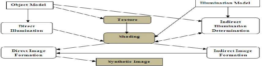
Image synthesis is the evolution of creating images from scenes is called rendering. This processing prepares the atmosphere for rendering [5] through such possessions as the propagation of energy throughout the environment or optimizations to demonstrate. An overview of general process as follows:
The object model is determined starting with those displaying procedure that we analyzed.
The Illumination model describes how light (and other energy components) is defined and managed.
Texture refers to the group of techniques (texture mapping, bump mapping, reflection mapping etc.) used to add effects to the surface of objects.
Shading refers to variations in plane lighting that result from the application of an illumination model.
[image:1.595.98.527.632.740.2] Image formation is the process of bringing together the other components to form a synthetic image, usually called rendering or image synthesis.
The applications of image synthesis are Computer - Aided Design (CAD), Entertainment, Simulation, Computer Art, Augmented Reality (Image analysis + Image Synthesis).
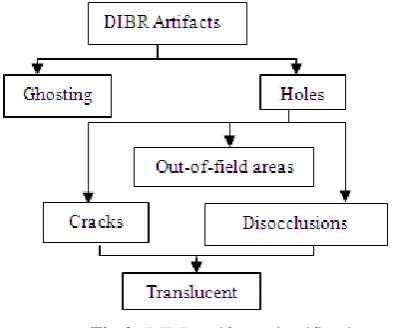
[image:2.595.56.254.232.396.2]The DIBR (Depth Image Based rendering) method has limitations due to inherent artifacts in the warped image [5]. As a result, perception of the depth and the desired experience are affected due to the reduced visual quality of virtual view. Rendering artifacts are severe in the extrapolated view, since there is no additional information to handle, whereas in the intermediate view the artifacts are partially filled with the information from the other warped view. Possible artifacts in the warped images are classified as shown in Fig 2. The artifacts in the warped image are ghosting and holes (i.e. uncovered areas).
Fig 2: DIBR artifacts classification
Ghosting artifacts are mixtures of colors at the edges in the original image which are projected into the neighbouring objects in the warped image. The cause of the ghosting artifact is the depth and texture misalignment and mixing of neighbouring colours at the depth discontinuities.
Holes are undefined pixels in the rendered images. They appear due to uncovered (not captured) regions because they were occluded by foreground in the original view. They are classified into three types, namely cracks, disocclusions and out-of field areas.
Cracks are one to two pixel-wide empty regions in the warped image. Cracks appear in the virtual view due to assigning warped pixel coordinate positions to the nearest integer coordinates.
Translucent cracks appear for the same reason as the cracks, but these areas possess background information as consequence of occlusions in virtual view.
Disocclusions [6] occur at depth discontinuities near the object borders. These are the result of regions being revealed in the virtual view as they have been occluded by the foreground in the original view. Therefore occlusions in the original view translate into disocclusions and appear as
holes in the virtual view as the result of the warping process. When there are more than two depth layers, we define foreground and background as relative terms. Occlusion areas between a relative foreground-background pair are referred to as overlaid occlusions. It is worth noting that the size of the disocclusions depends on the size of the baseline and the scene depth.
Translucent-disocclusions differ from common
disocclusions by exposing texture information that is present behind the relative background. Translucent disocclusions occur only when the depth has three or more layers, and where there are occlusions between layers. The magnitude of the disturbance created by translucent disocclusion artifacts depends on the placement of occlusions in the scene and the occlusion area. However, translucent disocclusion artifacts need to be addressed since they can deteriorate the perceived visual quality.
Out-of-field areas are also holes, which occur at image borders. They occur due to the limited field of view in the original view.
Unnatural contours are the pixilation of “new” edges between background and foreground in the warped image due to the colors of the pixels at the edge not being blended.
To reduce the DIBR artifacts a number of state-of-the-art solutions have been introduced. However, disocclusion handling still remains a challenging problem.
II. RELATED WORK
Image - based modelling[7] and rendering techniques have recently arriving with much attention as powerful substitute to usual geometry-based techniques for image synthesis. Instead of geometric primitives, a collection of sample images are worn to render novel views. Examples comprise the well known panoramas, light fields, and variants, concentric mosaics, etc. The reconstruction model (i.e., rendering) is treated as a multidimensional sampling problem, where new views are generated from compactly sampled images and depth maps instead of building precise 3D models of the scenes.
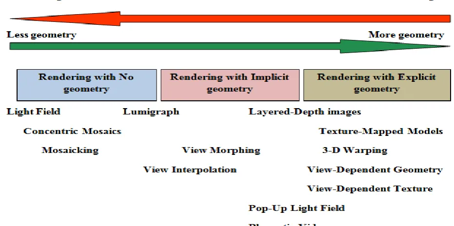
For instructive purposes, image – based representations can be classified according to the geometry information used into 3 main categories:
1) Representations with no geometry
2) Representations with implicit geometry
3) Representations with explicit geometry
2-D panoramas, 3-D concentric mosaics, 5-D McMillan and Bishop’s plenoptic modelling, 4-D ray-space representation, and light fields/ lumigraph belong to the first
category, while layered-based or object-based
Fig 3: Spectrum of IBR representations
At the other intense, light field or lumigraph rendering relies on opaque sampling (by capturing more image/videos) with no or very petite geometry information for rendering without recuperating the exact 3-D models. An important lead of the latter is its superior image quality, compared with 3-D model building for complex real world scenes and the other is that it requires noticeably less computational resources for rendering not considering of the scene complexity, because most of the quantities involved are precomputed or recorded. This has fascinated to considerable attention in the computer graphics community, recently in developing quick and efficient rendering algorithms for real-time relighting and soft shadow production.
Since capturing a 3-D model in real time is still a very difficult problem, light-field or lumigraph based dynamic IBR representations with slight amount of geometry information have received extensive attention in immersive TV (also called 3-D or multiview TV) applications. In particular, tremendous rendering quality has been demonstrated using the pop-up light field, the object-based approach and the layered based rendering approach. Later sections will be faithful to these representations, which use fairly accurate/ incomplete geometry in the appearance of depth maps. Segmentation, mapping, and depth estimation techniques are essential to these approaches.
On the other dispense, since 3-D models of the objects and scenes are not available, user communication is limited to the change of viewpoints and sometimes restricted amount of relighting. In contrast, more user interaction such as real-time relighting and soft-shadow computation has been found to be practicable using IBR concepts [8] and the associated 3-D models using precomputed shadow fields. This opens up a new chance for very fast interactive visualization /graphic systems with low complexity. If approximate geometry of objects in a scene can be recovered, then interactive editing and relighting of real scenes are in principle practicable. This has important applications in computer games, scientific visualization, and
relighting of IBR objects in future generations of IBR systems.
III. OVERVIEW
Texture is an important visual system and it is used to distinguish one object from other objects clearly. Especially in color images which provide extra information that can be used on its own or combined with texture information to segment images. Texture indexing is an act of classifying and in order to make items easy to retrieve.
On exposed area of an image do not have corresponding information about the reference view, their texture attributes are uncertain. Those uncertain values can be filled based on the neighbour pixels by linear interpolation [9], extrapolation [10] or inpainting [11].
Inpainting is one of the arts for restoring the lost or damaged parts of an image and also get rid of the unnecessary objects depending on the background of that image. This should be done in an untraceable way. Previously, in past days, the artists used to paint by their own manually of the damaged paints. As the technology is recuperating day to day, this image inpainting processes the inpainting automatically.
The subject of rendering which can be projection of environment into an image involves different subjects as we discussed here are object removal, occlusion culling and shadow removal.
A. Object Removal
The idea behind this part is to fill in larger areas of an image by repeating the textures that surrounds the target region with some level of stochasticity. This is done in an onion-peel like approach starting from the outer layers and moving inwards towards the centre of the target region.
linear systems, (ii) robustness to modifications in form of the goal region, (iii) balanced simultaneous structure and texture propagation all in single efficient set of rules as criminisi.
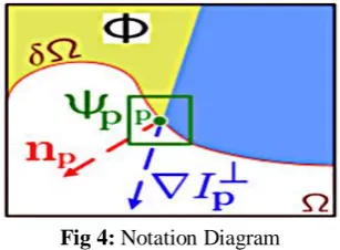
First, given an input image, the user selects a target region, Ω, to be removed and filled. The source region, Φ, may be defined as the entire image minus the target region (Φ = I − Ω), as a dilated band around the target region, or it may be manually specified by the user. Size of the template window Ψ must be specified as of 9×9 pixels, but in practice require the user to set it to be slightly larger than the largest distinguishable texture element, or “Texel”, in the source region.
In our criminisi algorithm [12], each pixel maintains a colour value (or “empty”, if the pixel is unfilled) and a confidence value, which reflects our confidence inside the pixel price, and which is frozen once a pixel has been filled. Throughout the course of the algorithm, patches alongside the fill the front are also given a transient precedence cost, which determines the order in which they may be filled. Then, our set of rules iterates the subsequent 3 steps till all pixels have been filled:
Fig 4: Notation Diagram
1. Computing patch priorities: The synthesis task through a best-first filling strategy that depends entirely on the priority values that are assigned to each patch on the fill front. The priority computation is based toward those patches which: (i) are on the continuation of strong edges and (ii) are surrounded by high-confidence pixels.
Given a patch Ψp centred at the point p for some p∈δΩ,
we define its priority P(p) as the product of two terms:
P(p) = C(p)D(p) (1)
We call C(p) the confidence term and D(p) the data term, and they are defined as follows:
C(p) = ∑q∈Ψp∩(I−Ω) C(q) /|Ψp|, (2)
D(p) = |∇Ip⊥·np| /α (3)
Where |Ψp| is the area of Ψp, α is a normalization factor
(e.g., α = 255 for a typical grey-level image), np is a unit
vector orthogonal to the front δΩ in the point p and ⊥ denotes the orthogonal operator. The priority P(p) is computed for every border patch, with distinct patches for each pixel on the boundary of the target region.
During initialization, the function C(p) is set to C(p) = 0 ∀p∈Ω, and C(p) = 1 ∀ p∈I−Ω. The confidence term C(p) may be thought of as a measure of the amount of reliable information surrounding the pixel p. The intention is to fill first those patches which have more of their pixels already filled, with additional preference given to pixels that were filled early on (or that were never part of the target region).
At a coarse level, the term C(p) of (1) approximately enforces the desirable concentric fill order. As filling proceeds, pixels in the outer layers of the target region will tend to be characterized by greater confidence values, and
therefore be filled earlier; pixels in the centre of the target region will have lesser confidence values.
The data term D(p) is a function of the strength of isophotes hitting the front δΩ at each iteration. This term boosts the priority of a patch that an isophote “flows” into. This factor is of fundamental importance in our algorithm because it encourages linear structures to be synthesized first, and, therefore propagated securely into the target region
2. Propagating texture and structure information: Once all priorities on the fill front have been computed, the patch Ψˆp with highest priority is found. We then fill it
with data extracted from the source region Φ.
On the contrary, we propagate image texture by direct sampling of the source region. Similar to, we search in the source region for that patch which is most similar to Ψˆp.
formally,
Ψˆq = arg min Ψq∈Φ d(Ψˆp,Ψq) (4)
Where the distance d(Ψa,Ψb) between two generic
patches Ψa and Ψb is simply defined as the sum of squared
differences (SSD) of the already filled pixels in the two patches. Pixel colors are represented in the CIE Lab colour space because of its property of perceptual uniformity. Having found the source exemplar Ψˆq, the value of each
pixel-to-be-filled, p|p ∈ Ψˆp∩Ω, is copied from its
corresponding position inside Ψˆq.
3. Updating confidence values: After the patch Ψˆp
has been filled with new pixel values, the confidence C(p) is updated in the area delimited by Ψˆp as follows:
C(p) = C(ˆp) ∀p∈Ψˆp∩Ω. (5)
This simple update rule allows us to measure the relative confidence of patches on the fill front, without image-specific parameters. As filling proceeds, confidence values decay, indicating that we are less sure of the color values of pixels near the centre of the target region.
A pseudo-code description of the algorithmic steps as follows:
Extract the manually selected initial front δΩ0.
Repeat until done:
1a. Identify the fill front δΩt. If Ωt =∅, exit. 1b. Compute priorities P(p) ∀p∈δΩt.
2a. Find the patch Ψˆp with the maximum priority,
i.e., ˆp = arg max p∈δΩt P(p).
2b. Find the exemplar Ψˆq ∈Φ that minimizes d(Ψˆp,Ψˆq). 2c. Copy image data from Ψˆq to Ψˆp ∀ p∈Ψp∩Ω. 3. Update C(p) ∀ p∈Ψˆp∩Ω.
The superscript ‘t’ indicates the current iteration.
Finally, pixels are classified as belonging to the target region Ω, the source region Φ or the remainder of the image by assigning different values to their alpha component. The image alpha channel is, therefore, updated (locally) at each iteration of the filling algorithm.
B. Occlusion culling
[image:4.595.88.242.309.422.2]depth data can be leveraged to produce higher quality, more accurate results.
The criminisi method and the proposed modified daribo method which simply added another term to the two main equations as:
( ) = ( ) ( ) ( ). (6)
L(p) is the level regularity term, or the inverse variance of the depth patch , described by:
L( ) =| | / [| | + ∑ ∈Ψ∩Φ ( − )2] (7)
Where | | is the area of and is the mean of . The level regularity term gives higher priority to patch overlaying at the same depth level, which naturally favours background pixels in the case of holes caused by disocclusions.
The best exemplar calculation went from minimizing the SSD of the known pixels of the target patch and patches of the known portion of the image to
Ψ q = arg min Ψ ∈Φ { (Ψ p, Ψ) + ∙ (Z p ,Z)} (8)
SSD of the target depth patch and all possible exemplar depth patches. With this new equation, we can control the importance of the SSD of the depth by changing the value of . They only considered depth pixels with values in their calculations, and their final product leaves the depth map full of holes.
Their algorithm fills the depth map prior to inpainting the image. This is done for two reasons: first, depth maps are usually constant or slowly changing, making them easier to fill, and second, the greater quantity of depth data assists in the image inpainting process. Ružić et al. [13] found that filling in entire rows of the depth map holes reasonably interpolates the depth data. Their algorithm fills the rows by extracting a suitable value from a local window located on the background side of the disocclusion hole.
During inpainting, all depth pixels are considered, and the top L best exemplars are averaged when filling in the target patch. Averaging the top exemplars adds a slight blur to the details added to the image, but it also helps prevent the algorithm from creating and propagating false structures in the image. The final change made is to limit the search area while the algorithm is checking for the best exemplar.
The method outperforms the depth-less Criminisi algorithm, where a premade mask was applied as the target area. Premade mask is part of the foreground, the background is automatically targeted first for inpainting, resulting in perfect reconstruction of original image.
C. Shadow removal
Shadows are ubiquitous in image and video data, and their removal is of concentration in both computer vision and graphics. Although shadows can be useful cues, e.g. shape from shading, they can also involve the performance of algorithms (e.g. in segmentation and tracking). Their removal and editing is also often the pain-staking task of graphical artists. An unbeaten shadow removal method should seamlessly relight the shadow area while keeping the lit area unchanged. The umbra is the darkest division of the shadow whilst the penumbra is the transitional shadow boundary with a non-linear intensity change between the umbra and lit area. The textures in shadowed surface generally become weaker that contrast artifacts can appear in shadow areas due to image post-processing.
The important contribution of this work is the first proven and multi-scene class ground truth for shadow removal algorithms. This data set containing 200 images
eliminates in consistencies between shadow and shadow-free images and provides a range of various shadow types such as soft, textured, colour and broken shadow. Using these facts, the most thorough comparison of state-of-the-art in user-aided shadow removal technique is performed.
A shadow image Ic may be taken into consideration as a
Hadamard product [14] of a shadow scale layer Sc and a
shadow-free image Ic as shown in Eq (9) where c is a RGB
channel. The scales of the lit area are 1 and other areas scales are between 0 and 1.
Ic = Ic * Sc (9)
For interactive shadow removal especially consists of 4 steps as Pre-processing, Penumbra Unwrapping, Relighting and Color Correction. Each step may be explained briefly with technical information for each of its components. In this we denote 6 undetermined parameters as h1,h2,...,h6.
1) Pre-processing
An initial shadow mask (Fig. 5(b)) is detected using a KNN classifier trained from data from two rough user inputs (e.g.Fig.5 (a)) are sample lit and shadow pixels. A fusion image, which magnifies illumination discontinuities around shadow boundaries, is generated by fusing channels of YCbCr color space and suppressing texture (Fig. 5(c)). Highlighted pixels RGB intensities in the Log domain are supplied as training features and used to construct a KNN classifier (K = 3). Euclidean distance is used as the distance measure and the majority rule with nearest point tie-break as the classification measure. Spatial filtering with a Gaussian kernel (size = h1, standard deviation =
h1/2
) is applied to the obtained image of posterior probability and binarize the filtered image using a threshold of 0.5 (e.g. Fig. 5(b)).To assist unwrapping of the penumbra, an image is derived that magnifies illumination discontinuities around the shadow boundary – also assisting penumbra location – which is called the fusion image (e.g. Fig. 5(c)). There are 2 steps in this process:
i) Magnification of illumination discontinuity We derive an initial fusion image F that maximises the contrast between shadow and lit areas by linearly fusing the three channels (Cl) of YCbCr space as eq.(10) as
follows:
3
1
l a C
F l l
subject to
3
1 1
l al
Where al is the fusing factor of Cl (positive). The best
fusing factors are derived by minimising the following objective function Eb:
)
(
/
))
(
)
(
(
)
(
/
)
(
)
(
L s L s L s bF
F
F
F
F
a
E
(11)where a is the vector of fusing factors and FS and FL are
the two sets of shadow and lit pixels marked by user scribbles. In this paper, σ and µ are defined as functions that respectively compute the standard derivation and mean of a set of values. The first term ensures larger distinction between pixels of lit and shadow regions and the second term ensures smaller variation for pixels of the same lit or shadow regions.
h2-by-h2 neighbourhood to F. YCbCr color space offers
perceptually meaningful information. Empirically,
illumination information appears dominantly in one of its
channels. The illumination information in RGB channels are usually affected by texture noise.
1) Pre-processing 2) Penumbra Unwrapping 3) Relighting 4) Color Correction
Fig 5: Our shadow removal pipeline. (a) input: a shadow image and user strokes (blue for lit pixels and red for shadowed pixels); (b) detected shadow mask; (c) fusion image; (d) initial penumbra sampling (the actual density of samples are higher than the displayed samples);(e) initial penumbra unwrap (only the shadow edges of the largest shadow segment is shown); (f) further aligned penumbra unwrap; (g) sparse shadow scale; (h) dense shadow scale; (i) initial shadow removal result; (j) color corrected shadow removal result; (k) ground truth.
2) Penumbra Unwrapping
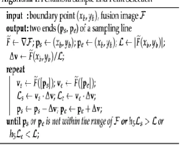
Based on the detection shadow mask and fusion image, pixel intensities of sampling lines are sampled perpendicular to the shadow boundary (Fig. 5(d)). Noisy samples are removed and remaining columns stored as the initial penumbra strip (Fig. 5(e)). The initial columns illumination changes are also aligned (Fig. 5(f)) by a fine-scale alignment.
The start and end points are initially set as the boundary point (xb,yb) and the direction vector ∆v as the
normalized gradient vector of (xb,yb). Instead of
processing unaligned and unselected samples individually, we transform these samples into unified columns of the initial penumbra strip to enable fast batch processing. And, only the good samples are kept for shadow scale estimation.
To avoid outliers, e.g. sampling lines at occlusion boundaries, invalid samples are filtered based on an
assumption of similar shadow scales. A scale vector Yc =
Tl −Ts is first computed where Tl and Ts are the average
Log-domain RGB intensities of the lit and shadow halves of a sampling line. Yc is then converted to spherical
coordinates and considered as feature vector Ys. DBSCAN
clustering [15] (radius: h3) is applied to Ys for all samples,
and samples that belong to the largest cluster are stored as valid ones with valid illumination. For finer scale estimation, valid clusters are further divided into a few sub-groups using mean-shift [16] (band width: h4) and the samples of invalid subgroups, whose total members are less than 10% of the largest sub-group’s, are discarded. Fig. 5(d) shows an example of the above outlier detection.
The parameters of this fine-scale alignment for each column are estimated by minimizing the following energy function Ea:
Ea = MSE(Ln−La) (12)
where Ln = Γ(As,Ak,Lo), whose As and Ak are the
stretching shift and the centre shift in the fine-scale alignment respectively, Lo is the scales of original column,
La is the reference of alignment which is the average scale
values of all valid columns (i.e. column-wise mean of the penumbra unwrap), Ln is the aligned unwrap, Γ is a
function that aligns Lo according to the estimated
alignment parameters, MSE is a function that computes mean squared error.
3) Relighting
[image:6.595.78.517.103.296.2] [image:6.595.39.225.490.640.2]A pyramid (e.g. Fig. 5(b)) of horizontally filtered penumbra unwraps using 5 averaging kernels in different sizes are computed so that texture noise can be cancelled. The sizes of averaging kernels are specified as 1-by-2˜n where ˜n∈{2,3,4,5,6}. The filtered intensities of the pyramid are then converted to shadow scales.
The optimum shadow scales for each column are selected from different layers of the pyramid. Column intensity with higher localness (i.e. filtered by a smaller kernel) and lower roughness are preferred. However, higher localness leads to higher roughness, so an optimum solution should balance these two properties. The roughness of intensity change Es(˜c, ˜n) is measured as
follows:
Es(˜c, ˜n) =∫(∂2u(˜r,˜c,˜n)/∂ ˜r2)2 d˜r (13)
Where u is the penumbra unwrap, ˜ n is the layer index of pyramid, ˜ c and ˜ r are the column and row coordinates of the penumbra unwrap respectively. The optimum scales for each column are selected using a threshold of roughness Ts which is computed as the mean of all values
in Es.
4) Color Correction
Post-processing effects may cause inconsistent tone and contrast in shadow removed areas compared with the lit areas. Without introducing additional artifacts, a multi-scale color correction is proposed to remove these inconsistencies (Fig. 5(j)).
Fig.6: Multi-scale color correction pipeline. The inconsistency in the initial shadow-free image (b) is fixed in the final output (f). The multi-scale color correction aligns the color variance at different scales from coarse to fine. On each single scale, the initial input image (c1) exhibits inconsistency of local variance between lit and shadow areas. The higher-frequency variation (c3) of shadow and lit areas are aligned in (c4). The corrected output (c5) can be obtained by adding (c4) to (c2).
Statistics are collected from the lit side pixels Pl and
the umbra side pixels Pu both near the penumbra as the
reference and source of color correction respectively. The algorithm for alignment is described in Algorithm2. Where s is a scale, β is the maximum image dimensional of Ira, bfilter is an operation that bilaterally filters [17] the input image (first parameter) using a standard deviation of the space (second parameter) and a range Gaussian (third parameter), Ih is an image of
intensity variation, where c is the channel index, m is a function which computes the median absolute deviation.
Finally, to smooth the color correction result, alpha blending is applied in RGB color space according to the shadow scale as shown in Eq. (14).
Icf = Icr Sc + Icra (1− Sc) (14)
Where c is the channel index, Sc is the normalized
scale field of S, Icf is the final shadow-free image. An
5) Error Measurement
Our objective function Ep minimizes the sum of all error
measurements as the follows:
k
w
e
H
E
p(
)
k k (15)Where ek is the kth error measurement and wk is the
weight for ek. We assume that the weights for all error
measurements are the same (i.e. equally important), e.g., wk
[image:8.595.68.526.168.254.2]= 1. Table 1 shows the details of these parameters and their optimization configuration. In our experiment, 5 test cases are randomly selected for computing each error measurement. The optimum parameters for all error measurements are learned as [14 10 0.1124 0.0333 8.5195 0.2228].
Table 1. Parameter learning specification for the optimization.
ID Description Range Initial value Type
h1 h2 h3 h4 h5 h6
Gaussian filter Kernel size(C.1)) medium filter Kernel size (C.1)) DBScan Radius (C.2))
meanshift Radius (C.2)) gradient advance scale (Alg. 1) bilateral filter sampling spatial (Alg. 2)
[image:8.595.58.261.470.712.2][2, 15] [2, 15] [0.01, 0.5] [0.01, 0.5] [2, 20] [0.1, 0.3]
5 10 0.2 0.06 10 0.2
Int. Int. Real Real Real Real
D. Evaluation
In this section, we first describe experiments that highlight our algorithms behaviour given variable user inputs. The quality of our new ground truth versus existing state-of-the-art ground truth is then quantitatively evaluated. Finally, our algorithm is evaluated versus other state-of-the-art shadow removal methods based on our new dataset.
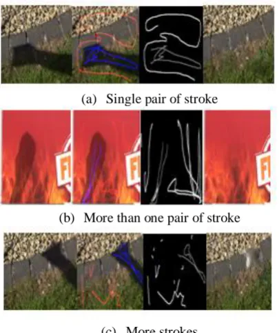
Given user-supplied single pairs of strokes of lit and shadow pixel samples, our shadow detection generates stable results in different conditions (e.g. Fig. 7(a)). In some cases, e.g. where the surface color is very shadow-like, the detection results can be improved by supplying more than one pair of strokes (e.g. Fig. 7(b)).
Fewer gray pixels indicate higher stability, i.e. the image should only show black (0% probability) and white (100% probability) pixels when it is absolutely stable. The bottom row shows examples highlighting how additional strokes can improve the detection result (binary mask).
(a) Single pair of stroke
(b) More than one pair of stroke
(c) More strokes
Fig 7: Rougher stroke requirement: To generate a reasonable shadow removal result, our method requires less input strokes (in the same format).
1) Ground Truth Quality
Ideal pairs of ground truth images should have a minimum intensity difference in the common lit area – which will also indicate whether registration is poor (due to camera shake or scene movement – which should be rejected). This is utilized to assess the quality of ground truth candidates. The error image ∆I = Is −Ig and the ratio
image Ir = Φ(Is) ø Φ(Ig) are first computed, where Is and Ig
are the original shadow image and its shadow-free ground truth image (which differs from the processed shadow-free outputs If in Eq. 14) respectively, ø is element-wise division and Φ is a function that converts RGB image to gray-scale image. The set of pixels Pr of Ir that satisfies Ir(Pr) ≥1 are
regarded as lit pixels. Due to some unavoidable minor global illumination changes and the inaccuracy in camera exposure control, the lit intensities in the shadow image can be higher than those in the shadow-free ground truth image. Ir can therefore be greater than 1. The ground truth error Qd
is computed as follows:
Qd = µ(|∆I(Pr)|) + σ(∆I(Pr)) (16)
Ground truth pairs in our data set with Qd > 0.05 are
removed. To test robustness, the standard deviation for each measurement is also computed. Unlike previous un-categorized test, our removal test is based on our data set of 214 cases, which contains challenging soft, broken and color shadows and shadows cast on strong textured surfaces. Each case is rated according to 4 attributes, which are texture, brokenness, colourfulness and softness, in 3 perceptual degrees from weak to strong which were aggregated by 5 users.
2) Quantitative evaluation of shadow removal The quality of shadow removal is measured by directly using the per-pixel error between the shadow removal result and shadow-free ground truth. However, a shadow in a smaller size or a lighter shadow can result in a smaller initial error between the original shadow image and its shadow-free ground truth. It is thus unfair to judge that a method is better only because the error between the shadow removed image and its shadow-free ground truth is smaller. In our work, we cancel out the affects of the size and darkness of the shadow. We therefore compute the error ratio Er as our
quality measurement:
Where En is the error between the ground truth (no
shadow) and shadow removal result, and Eo is the error
between the ground truth (no shadow) and the original shadow image. This normalized measure better reflects
removal improvements towards the ground truth
independent of original shadow intensity and size. We assess En and Eo using Root-Mean-Square-Error (RMSE) of
RGB intensity. According to Eq. 17, Eo for all pixels is
lower than Eo for the shadow pixels only because the
intensity errors of the lit pixels are close to 0 and Eo
measures the RMSE. In addition, the new RMSE En for both
all pixels and shadow pixels only are very close after shadow removal, the error ratio Er for the shadow pixels
only is therefore generally lower.
Our method requires users to supply reasonable inputs. We have not considered its tolerance for very careless user inputs (e.g. mistakenly marking many shadow pixels as lit samples). Besides, insufficient user inputs may result in poor shadow detection. Since a sufficiently trained shadow classifier may be robust to this issue, another future work could be improving shadow detection by combining user inputs with the shadow masks generated from an automatic shadow classifier.
IV. CONCLUSION
We have presented a texture mapping based on uncertain values of neighbour pixels by inpainting concentrated on rendering artifacts of occlusions and a number of state-of-the-art solution in case of user-aided shadow removal method is performed using matlab. Occlusion culling method utilizes aspects of several disocclusion inpainting methods to achieve desirable and visually believable results. It consistently outperforms a similar function which does not consider depth information. Shadow removal of our technique balances the complexity of user input with sturdy shadow removal performance. Our quantitatively-verified ground truth data set overcomes issues of mismatched illumination and registration in present data sets. Except the opportunities for improving shadow removal quality for the categorized shadows in our dataset, the detection and elimination for fantastically-complex shadows, such as overlapping shadows precipitated multiple mild resources with one of kind mild colors, and shadows as a result of transparent gadgets with complex internal shape and color, continues to be an open trouble for the community.
V. REFERENCES
[1] H. C. Longuet-Higgins, “Readings in computer vision: issues, problems, principles, and paradigms,” chapter A computer algorithm for reconstructing a scene from two projections, pp. 61–62. Morgan Kaufmann Publishers Inc., San Francisco, CA, USA, 1987. [2] L. Liang, C. Liu, Y.Q. Xu, B. Guo, and H.Y. Shum,
“Real-time texture synthesis by patch-based sampling”, In Proc. ACM Transactions on Graphics, 2001.
[3] Foley, J. D., Van Dam, A., Feiner, S. K., and Hughes, “Computer Graphics: Principles and practice”, Addison-Wesley, Reading, Massachusetts, 1990. [4] P. Debevec, Y. Yu, and G. Borshukov, “ Efficient
view-dependent image-based rendering with projective
texture-mapping”, In Proc. 9th Eurographics
Workshop on Rendering, pp. 105–116, 1998.
[5] X. Xu, L. M. Po, C. H. Cheung, L. Feng, K. H. Ng, K. W. Cheung, “Depth-aided Exemplar-based Hole Filling for DIBR View Synthesis”, In Proc. IEEE International Symposium on Circuits and Systems, Beijing, China, pp. 2840-2843,2013.
[6] S. M. Muddala, M. Sjostrom and R. Olsson, “Depth-Based Inpainting for Disocclusion Filling”, In Proc. 3DTV-Conference: The True Vision - Capture, Transmission and Display of 3D Video, Budapest, Hungary, pp. 1-4,2014.
[7] GRZESZCZUK, R. 2002.Course 44: Image-based modeling. In Proc. SIGGRAPH, 2002.
[8] S. B. Kang, “ A survey of image-based rendering techniques”, In Proc. VideoMetrics, SPIE Vol. 3641, pp. 2–16, 1999.
[9] Chen. S, and Williams. L, “View interpolation for image synthesis”, In Proc. SIGGRAPH, pp. 279–288, Aug-1993.
[10] Lai-Man Po, Shihang Zhang, Xuyuan Xu, Yuesheng Zhu, “A new multidirectional extrapolation hole-filling method for depth-image-based rendering”, In Proc.
IEEE International Conference on Image
Processing,2011
[11] M. Bertalmio, G. Sapiro, V. Caselles, and C. Ballester, “Image inpainting”.In Proc. ACM Conf. Comp. Graphics (SIGGRAPH), pp. 417–424,New Orleans,
LU, Jul-2000.
http://mountains.ece.umn.edu/~guille/inpainting.htm. [12] A. Criminisi, P. Perez, and K. Toyama, “Object
removal by exemplar-based inpainting”, In Proc. Conf. Comp. Vision Pattern Rec., Madison, WI, Jun- 2003. [13] Ruzic, T.; Jovanov, L.; Hiep Quang Luong; Pizurica,
A.; Philips, W.,"Depth-guided patch-based
disocclusion filling for view synthesis via Markov random field modelling," In Proc. In Signal Processing
and Communication Systems (ICSPCS), 8th
International Conference, pp.1-9, 15-17, Dec- 2014. [14] H. Barrow and J. Tenenbaum, “Recovering intrinsic
scene characteristics,” Computer Vision System, A Hanson & E. Riseman (Eds.), pp. 3–26, 1978.
[15] M. Ester, H.-P. Kriegel, J. Sander, and X. Xu, “A density-based algorithm for discovering clusters in large spatial databases with noise”, In Proc. KDD , vol. 96, pp. 226–231,1996.
[16] D. Comaniciu and P. Meer, “Mean shift: A robust approach toward feature space analysis,” In Proc. IEEE Transaction on Pattern Analysis and Machine Intelligence, vol. 24,Issue 5, pp. 603–619, 2002. [17] S. Paris and F. Durand, “A fast approximation of the