Volume 6, No. 6, July-August 2015
International Journal of Advanced Research in Computer Science
RESEARCH
PAPER
Available Online at www.ijarcs.info
A New Partition Based Association Rule Mining Algorithm for BigData
P.Prabakaran
Research Scholar, Department of computer science, Mass college of arts and science, Kumbakonam, Tamilnadu, India.
Dr.K.RameshKumar, Ph.D.,
Research supervisor & Assistant professor Department of computer science, Mass college of arts and science, Kumbakonam, Tamilnadu, India,
Abstract: Association Rule Mining is an important research area in the field of Data Mining especially in case of ‘Sales transactions’. A number of algorithms have been presented in this regard. In this paper a comparison of PARTITION algorithm with CMA algorithm is presented after improving the PARTITION algorithm. In this study, randomized partitioning of database is done. The database is randomized so that real random data is available for better results. The randomized partitioning of database has been implemented in different tool, i.e., VB. Net, as compared to CMA, which uses MATLAB for randomization so as to achieve better performance and efficient results. In the end it has been proved with extensive experiments that although Randomized PARTITION algorithm takes two database scans as compared to CMA that takes single database scan, still it gives better results with more efficiency than CMA.
Keywords: Data Mining, Association Rule Mining, Randomized PARTITION Algorithm
I. INTRODUCTION
In the past few years the amount of data in business organizations has been increased to a greater extent, so the extraction of useful information from such databases is an uphill and challenging task. Data mining techniques can be applied in various fields like sales transaction, marketing, finance, insurance, medicine and fraud detection etc. Interesting association relationships are much helpful in taking good business decisions like how to increase sales or purchases process. Its basic aim is to analyze entire huge database to find the frequently occurring item sets together. For the rule generation it takes one or multiple scans of the whole database. Association rule mining can be best explained by a simple example of market basket analysis that basically determines which groups of products or items are sold or purchased together most frequently at the same time. Customer buying behavior can be best analyzed by this process, as it helps in finding association among different item sets. For example if customers buy soft drink and chips together mostly with in the same visit to the superstore then using this information for the next time the shop keeper will place the soft drink and chips in the nearer shelves. Such shelf arrangement of these items will increase the sales process in future visits to the store. Similarly if a person orders a birthday cake to some bakery, then he is likely to be purchasing some birthday candles as well. If the baker is aware of the association between candles and the birthday cake then he must be offering his customers to purchase candles from him, hence supporting his candle business as well. Market basket analysis is helpful for the retailers in the best adjustments of catalogue design and store layouts etc.
In this study an improved version of PARTITION algorithm is presented and it has been proved through various experiments that its performance is much better than previously implemented PARTITION algorithm as it reduces the memory usage as well as time. Its efficiency is also compared with previously implemented CMA
algorithm and it has been proved that due to its efficient partitioning technique of database it gives better results than CMA in terms of time efficiency.
EXISTING RULE MINING ALGORITHMS
Association rule mining for the first time was introduced by Agrawal et. al. (1993). It has remained highly in use by the pundits and practitioners of the data mining for more research since its inception. Many algorithms have been discovered in this field. According to Han and Kamber (2001), association rule mining searches for the interesting relationships among the items in a given dataset. For example, if the support = 5%, confidence=70%. Association rule for the last discussed example of birthday cake and candle is:
Birthday cake => candles
Rule interestingness can be measured well by support and confidence. Support=5% shows that for the above discussed rule, the birthday cake and candles are bought together in all transactions. Confidence=70% means that 70% of the customers who buy a birthday cake also purchased birthday candles.
Association rule mining basic concept as illustrated by Han and Kamber (2001) is as follows: Let I = {i1,i2,…,im}
be the set of items. Let D, the task-relevant data, is a set of database transactions where each transaction T is a set of items such that T ⊂ I. Each transaction is associated with an identifier TID. Let A be a set of items. A transaction T is said to contain A if and only if A⊂ T. An association rule is an implication of the form A⇒B, where A ⊂ I, B ⊂ I, and A∩B = φ. The rule A⇒B holds in the transaction set D with support s, where s is the percentage of transactions in D that contain A U B (i.e., both A and B). This is taken to be the probability, P (AUB). The rule A⇒B has confidence c in the transaction set D if c is a percentage of transactions in D containing A that also contain B. This is taken to be the conditional probability, P (B|A). That is,
Confidence (A⇒B) = P (B|A). (2)
Rules that satisfy both a minimum support threshold (min_sup) and a minimum confidence threshold (min_conf) are called strong. By convention, we write support and confidence value so as to occur between 0% and 100%, rather than 0 to 1.0.
Association rule mining is a two-step process. Firstly, find all frequent itemsets: by definition, each of those itemsets will occur at least as frequently as a pre-determined minimum support count. Secondly, generate strong association rules from the frequent itemsets: by definition, these rules must satisfy minimum support and minimum confidence. The association rules are generated simply using the following formula:
If (support ({Y, X})) ≥ min_conf. (3) support ({X})
Then X⇒Y is a valid rule.
Here X is called the antecedent of the rule, whereas Y makes the consequent of the rule.
Many algorithms have been discovered in this field. The pioneer work in this area was presented by Agrawal and Srikant (1994). They discussed Apriori algorithm. Apriori is termed as the best base algorithm for all other subsequent algorithms. Apriori was an iterative algorithm which used complete bottom search to find out large 1-itemset in first pass. Next pass generated candidate itemsets and checked the support. The process repeated until all large itemsets were found. Other variants of Apriori, AprioriTid and AprioriHybrid were also discussed by them in the same paper. In Apriori for n iterations, n scans of the entire database were done. AprioriTid overcame this problem in later iterations, as it did not use the whole database for counting support after the first pass. Best features of both Apriori and AprioriTid were combined in AprioriHybrid which showed good performance than the other two in real applications.
DHP (Direct Hashing and Pruning) algorithm was presented by Park et. al. (1995), which was an extension of Apriori algorithm. It was confined to the generation of large itemsets, the step one of the mining association rules. The problem with this algorithm was that database pruning benefit was quite ambiguous.
Zaki (1999) presented the survey of parallel and distributed association rule mining algorithms. These algorithms were divided into groups according to the techniques utilized, database structure and search techniques etc. This paper also provided the design space of parallel and distributed algorithms either implemented on distributed or shared–memory architecture. The aim of this paper was to provide a reference for more research. It also described the challenges and problems in the field of association rule mining.
Savasere et. al. (1995) presented PARTITION algorithm that worked in two phases. Logical division of horizontal database into non-overlapping partitions was done. Then locally large itemsets were found for each partition. For each locally large itemset, the TIDs were stored in hash tree. Further potentially large itemsets were obtained by merging the locally large itemsets at the end of phase I. To find the globally large itemsets actual support of these itemsets was measured in phase II. For the available
memory to uncover accurate no. of partitions was unsolvable by this algorithm.
Jamshaid et. al. (2007) implements CMA (Centralized Mining of Association-Rules) algorithm for association rule mining. In this algorithm the database was divided into logical non overlapping partitions and then DMA algorithm was applied on each partition to find local and global large itemsets. This algorithm took just a single database scan over each partition for the creation of large itemsets.
From the literature review it is concluded that despite the recent advances in association rule mining algorithms, there are still some problems like in large databases, scanning is much expensive and the resulting candidate itemsets are too large to fit in the aggregate memory. Data skew, data size, multiple scans and pruning techniques needs further study.
PROPOSED NEW RANDOMIZED PARTITION ALGORITHM
In this paper, Randomized PARTITION algorithm has been implemented. Logical non overlapping partitions are created with both random and non random data. Results of both randomized and non randomized partitions are compared to see the effect of data skew on both locally and globally large itemsets. Then the efficiency of Randomized PARTITION algorithm is compared with CMA.
PARTITION algorithm was previously implemented in Silicon Graphics Indy R4400SC workstation with a clock rate of 150 MHz and 32 Mbytes of main memory. The data resided on 1GB SCSI presented by Savasere et. al. (1995).
In this study Randomized PARTITION algorithm has been implemented in the same environment as CMA except the partitioning of database that has been done in a different tool (i.e. CMA has used .NET while Randomized PARTITION algorithm is using MATLAB) for achievement of better performance and efficient results. This change in partitioning technique increases the time efficiency of algorithm as compared to CMA. In today’s world, time is an important factor. Along with the need of accurate results, time efficiency matters a lot. It is important to have better results in less time and minimum cost. Randomized PARTITION algorithm has also been improved by using count structure rather storing TIDs in Hash tree as was done in previously implemented PARTITION algorithm. This change reduces the high memory usage and time as compared to previously implemented PARTITION algorithm.
Synthetic database is used for this study which is the same database as was used by CMA. It is also assumed that transactions are in the form (TID, i1, i2, i3). The items are
assumed to be kept sorted in lexicographic order. Similar assumption is also made by Han and Kamber (2001).
Algorithm
//Read database sequentially Read_Database
P=Create_Partitions (rand) For x=1 to P
Begin
Generate_Candidate_Itemsets Ci for px
//Generate local large itemsets Li for pi from Ci and store
items and their count in structure Si
Si=Gen_Local_Large_Itemset Li
End
//store value in global candidate structure
Merge local large itemsets to form global candidate itemsets Gi_C
End
//Generate globally large itemsets Gi from Gi_C
Gi=Gen_Global_Large_itemset (Gi_C)
Table 1: Notations Used
Notations Definition
Px Partitions (x=1 to 4)
Ci_L Local candidate itemsets
Li Local large itemsets
Si Structure for storing local large itemsets along
with their counts in particular partition pi
Gi_C Global candidate itemsets containing local large
itemsets along with their counts
Gi Globally large itemsets
* Not possible
Working of Randomized Partition Algorithm
First of all database is read in sequential order. Then logical non overlapping randomized or non randomized partitions are created. Partition size is chosen in such a way that for a specific time a whole partition can easily reside in memory. Partition size should not be very small or very large, as small partitions are negatively affected by data skew and in large partitions for intermediate results processing buffer requirements can exceed the available space, so risk is involved in both cases. Candidate large 1 itemsets are generated for all partitions. Then local large 1 itemsets are generated containing items having their support greater than user defined minimum support within each partition and the candidate itemsets whose minimum support is less than user defined minimum support are pruned away. Here a count structure is used for large itemsets rather than storing TIDs in a Hash tree. Storage of TIDs in hash tree is wastage of time and memory that’s why count structure is used for finding large itemsets directly. These large itemsets are then merged and stored in global candidate 1 itemset along with their counts for the generation of globally large itemsets. From large 1 itemsets, candidate large 2 itemsets are generated from which local large 2 itemsets are generated for each partition. The process continues upto locally large k itemset generation. Finally globally large itemsets are generated and global candidate itemsets having minimum support less than user defined minimum support are pruned away. Randomized PARTITION algorithm reduces the time complexity up to O (n) as compared to CMA whose time complexity is O (n3). Experimental results proved that Randomized PARTITION is 3 times more efficient than CMA.
A. Functions Of Randomized Partition Algorithm:
Function [T] = Read_Database
Reads the entire database sequentially and returns the transactions in an array.
Function [P] = Create_Partitions (rand)
This function takes rand as argument. If rand=0 then sequential (non randomized) non overlapping partitions are created otherwise T is first randomized and then logical non
overlapping partitions are created and an array of partition P is returned.
Function [LocalLargeItemset] = Generate_Large_Itemsets (pi)
This function creates candidate itemsets for all partitions and then from these candidate itemsets local large itemsets are generated for each partition. This function returns locally large itemsets for each partition.
Function [GlobalCandidate] = Generate_Global_Candidate (LocalLargeItemsets)
This function takes LocalLargeItemsets as an argument, merge them and generates global candidate itemset.
Function [GlobalLargeItemset] = Generate_Global_Itemsets (GlobalCandidate)
This function takes GlobalCandidate as an argument and generates globally large itemsets RIP.
B. Explanation of Randomized Partition Algorithm
with Example:
Performance of Randomized PARTITION algorithm can be best demonstrated by the case study. Following dataset was used for the case study: The dataset shown in Table II was randomized as shown in Table III to find out large itemsets. The results generated by this dataset are shown in Table IV. For testing the algorithm, many experiments were performed by taking both random and non random data. Number of items in the given dataset was 5.
Initially, the database was read sequentially and four logical non overlapping partitions were created. Then local and global itemsets for sequential database partitions were generated. In the second step, the database was randomized and again logical non overlapping partitions (P1, P2, P3, P4)
were created. After partition creation, the Randomized PARTITION algorithm was applied to find locally large 1-itemsets for each partition. From this, candidate 2-itemset was generated and then locally large 2-itemset for each partition was created. This process continued unless up to k large itemsets were found. The algorithm stored counts of the locally large itemsets in a structure rather than using a hash tree for this process. This change reduced the high memory usage as compared to previously implemented PARTITION algorithm. Then large itemsets of all lengths were merged to produce global candidate itemsets from which the globally large itemsets of all lengths were generated. Table V shows the experimental results of randomized and non-randomized partitions with 100 transactions.
implemented PARTITION algorithm and it was observed that its efficiency is better in terms of memory usage and time as shown in Table VIII. Extensive experiments were
[image:4.595.112.486.129.613.2]performed with different datasets for large itemset generation upto k itemset to check the efficiency of algorithm.
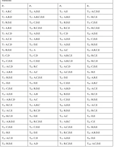
Table 2: Sequential Dataset
Partitions
P1 P2 P3 P4
T1: A,B,C T26: A,D,E T51: A,E T76: A,C,D,E
T2: A,B,D T27: A,B,C,D,E T52: A,B,E T77: B,C,E
T3: B,D,E T28: C,D,E T53: B,D,E T78: C,D,E
T4: A,B,E T29: B,C,D,E T54: B,C,E T79: B,C,D,E
T5: A,C,D T30: A,D,E T55: C,D T80: A,D,E
T6: A,C,E T31: A,B,E T56: A,D,E T81: C,D,E
T7: A,C,D T32: D,E T57: A,D,E T82: B,D,E
T8: B,D,E T33: A T58: A,C T83: A,B,C,E
T9: C,D T34: C,D T59: A,B,C,E T84: B,C,E
T10: C,D,E T35: C,D,E T60: A,B,C,D T85: B,C,D
T11: A,C,D T36: B,C T61: A,C,D T86: C,D,E
T12: A,B,E T37: A,C T62: A,C,D,E T87: B,E
T13: B,D,E T38: A,C,D,E T63: D,E T88: A,B,E
T14: D,E T39: D,E T64: C,D,E T89: A,B,C
T15: C,D,E T40: B,D,E T65: A,B,D T90: A,C,E
T16: A,D,E T41: A,B T66: B,D,E T91: B,C,E
T17: A,B,C,D T42: A,C T67: C,D,E T92: B,D,E
T18: B,C,E T43: A,B,C T68: A,D,E T93: A,C,E
T19: A,C,E T44: B,C,D T69: B,D,E T94: B,C,E
T20: B,C,D T45: D,E T70: A,C T95: D,E
T21: A,B,D,E T46: B,C,D,E T71: A,B,C T96: C,E
T22: C,D,E T47: C,D,E T72: A,C,D,E T97: B,D,E
T23: B,E T48: D,E T73: B,C,D,E T98: A,B,D,E
T24: A,C,D T49: C,D T74: A,D,E T99: D,E
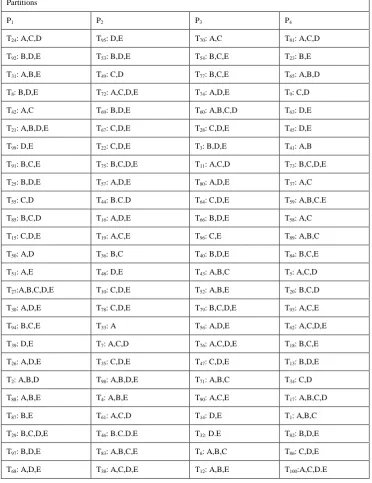
Table 3: Randomized Dataset
Partitions
P1 P2 P3 P4
T24: A,C,D T95: D,E T70: A,C T81: A,C,D
T92: B,D,E T53: B,D,E T54: B,C,E T23: B,E
T31: A,B,E T49: C,D T77: B,C,E T65: A,B,D
T8: B,D,E T72: A,C,D,E T74: A,D,E T9: C,D
T42: A,C T69: B,D,E T60: A,B,C,D T63: D,E
T21: A,B,D,E T67: C,D,E T28: C,D,E T45: D,E
T99: D,E T22: C,D,E T3: B,D,E T41: A,B
T91: B,C,E T75: B,C,D,E T11: A,C,D T73: B,C,D,E
T25: B,D,E T57: A,D,E T80: A,D,E T37: A,C
T55: C,D T44: B.C.D T64: C,D,E T59: A,B,C.E
T85: B,C,D T16: A,D,E T66: B,D,E T58: A,C
T15: C,D,E T19: A,C,E T96: C,E T89: A,B,C
T50: A,D T36: B,C T40: B,D,E T84: B,C,E
T51: A,E T48: D,E T43: A,B,C T5: A,C,D
T27:A,B,C,D,E T10: C,D,E T52: A,B,E T20: B,C,D
T30: A,D,E T78: C,D,E T79: B,C,D,E T93: A,C,E
T94: B,C,E T33: A T56: A,D,E T62: A,C,D,E
T39: D,E T7: A,C,D T76: A,C,D,E T18: B,C,E
T26: A,D,E T35: C,D,E T47: C,D,E T13: B,D,E
T2: A,B,D T98: A,B,D,E T71: A,B,C T34: C,D
T88: A,B,E T4: A,B,E T90: A,C,E T17: A,B,C,D
T87: B,E T61: A,C,D T14: D,E T1: A,B,C
T29: B,C,D,E T46: B.C.D.E T32: D.E T82: B,D,E
T97: B,D,E T83: A,B,C,E T6: A,B,C T86: C,D,E
Table 4: Results of Local and Global Itemset Generation
Local Large itemsets (Li) Global Large
Itemset (Gi) P1
Item = Count
P2
Item = Count
P3
Item = Count
P4
Item = Count
Gi
Item = Count
L1:B=14 D=18, E=19 L2:* L3:* L4:* L5:*
L1:C=16 D=19, E=19
L2:DE=17
L3:* L4:* L5:*
L1:C=15 D=15,
E=20 L2:* L3:* L4:* L5:*
L1:C=18 D=15 E=14 L2:* L3:* L4:* L5:*
G1:D=52 E=72 G2:* G3:* G4:* G5:*
Table 5: Comparison of number of large itemsets of randomized and non randomized datasets
Sequential Randomized 1 Randomized 2 Randomized 3
ΣLi P Gi ΣLi P Gi ΣLi P Gi ΣLi P Gi
L1=14 L2= 1 L3= * L4= * L5= *
G1=3 G2=* G3=* G4=* G5=*
L1=12 L2= 1 L3= * L4= * L5= *
G1=2 G2=* G3=* G4=* G5=*
L1=12 L2= 1 L3= * L4= * L5= *
G1=2 G2=* G3=* G4=* G5=*
L1=11 L2= 2 L3= * L4= * L5= *
G1=2 G2=* G3=* G4=* G5=*
Table 6: Comparison of Randomized Partition with CMA
CMA Randomized PARTITION
Time complexity of Partitioning database=O(n3)
Time complexity of algorithm after partitioning=O(n3)
[image:6.595.61.537.346.558.2]Time complexity of Partitioning database=O(n) Time complexity of algorithm after partitioning=O(n)
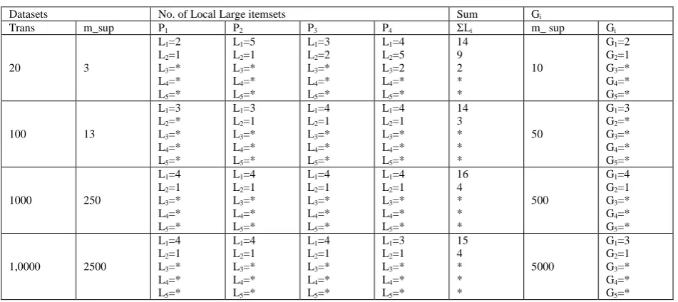
Table 7: Comparison of number of large itemsets with variable size of data
Datasets No. of Local Large itemsets Sum Gi
Trans m_sup P1 P2 P3 P4 ΣLi m_ sup Gi
20 3
L1=2 L2=1 L3=* L4=* L5=*
L1=5 L2=1 L3=* L4=* L5=*
L1=3 L2=2 L3=* L4=* L5=*
L1=4 L2=5 L3=2 L4=* L5=*
14 9 2 * * 10
G1=2 G2=1 G3=* G4=* G5=*
100 13
L1=3 L2=* L3=* L4=* L5=*
L1=3 L2=1 L3=* L4=* L5=*
L1=4 L2=1 L3=* L4=* L5=*
L1=4 L2=1 L3=* L4=* L5=*
14 3 * * * 50
G1=3 G2=* G3=* G4=* G5=*
1000 250
L1=4 L2=1 L3=* L4=* L5=*
L1=4 L2=1 L3=* L4=* L5=*
L1=4 L2=1 L3=* L4=* L5=*
L1=4 L2=1 L3=* L4=* L5=*
16 4 * * * 500
G1=4 G2=1 G3=* G4=* G5=*
1,0000 2500
L1=4 L2=1 L3=* L4=* L5=*
L1=4 L2=1 L3=* L4=* L5=*
L1=4 L2=1 L3=* L4=* L5=*
L1=3 L2=1 L3=* L4=* L5=*
15 4 * * * 5000
G1=3 G2=1 G3=* G4=* G5=*
Table 8: Comparison of previous partition with randomized partition algorithm
Previous PARTITION Randomized PARTITION
Memory usage=increased Hash tree storage
Memory usage=decreased Structure with count
IV. CONCLUSION
This improved version of Randomized PARTITION algorithm is more efficient than CMA as its partitioning technique takes much less time than the one used by CMA. Its time complexity is O (n) much better than the time complexity of CMA that is O (n3). Its efficiency is greater than CMA due to its changed partitioning technique. This version of Randomized PARTITION algorithm is also more efficient than previously implemented PARTITION algorithm as it reduces the memory usage by simply storing counts for each large itemset instead of storing the TIDs in hash tree. This has also increased the time efficiency of
Randomized PARTITION algorithm as compare to previously implemented PARTITION algorithm. In future we have a plan to implement this algorithm in parallel environment for better efficiency.
V. REFERENCES
[1] Han, J. and M. Kamber, 2001,Data Mining: concepts and Techniques. Kaufmann Publishers, San Francisco, Calfornia, USA, 2001.
[2] Agrawal, R., T.Imielinski, and A. Swami, 1993. Mining Association Rules between Sets of Items in Large Databases. In Proceedings of the ACM SIGMOD International Conference on Management of Data, Washington, D.C.USA, May 1993, pp.207-216.
Santiago de Chile, Chile, September 1994, edited by J.B.Bocca, M.Jarke, and C.Zaniolo, “Very Large Data Bases”, Morgan Kaufmann Publishers, San Francisco, CA, USA, pp. 487-499.
[4] Park. J.Soo, M. Chen and P.S.Yu, 1995. An Effective Hash-Based Algorithm for Mining Association Rules. In Proceedings of the ACM SIGMOD International Conference on Management of Datga, May 1995, pp.175-186.
[5] Zaki, M.J.1999. Parallel and Distributed Association Mining: A Survey. In EEE Concurrency Journal, Special
issue on Parallel Mechanisms for Data Mining, Vol.7, No.4, December 1999, pp.14-25.
[6] Savasere, A.E. Omiecinski and S.Navathe, 1995. An Efficient Algorithm for Mining Association Rules in Lagre Databases, In Proc. Of the 21st Int’l VLDB Conference, Zurich, Switzerland, September 1995, pp.432-444.