!
"
#"#
$ % %#
&
'
((( )
An Effect of Single Point Inversion Operator on the Performance of Genetic Algorithm
for Operating System Process Scheduling Problem
Er. Rajiv Kumar*
PhD. Scholar Singhania University Jhunjhunu,Rajasthan, India [email protected]
Er. Sanjeev Gill
Lecturer, Civil Engg. Deptt.
Global research Institute of Management & Technology Radaur Yamuna Nagar,Haryana India
Er.Ashwani Kaushik
Lecturer,Mechanical Engg Deptt. N.C.College of Engineering Israna, Panipat India
Abstract: Genetic algorithm is a Mata-heuristic search technique; this technique is based on the Darwin theory of Natural Selection. This algorithm is work with some finite set of population. The population contain set of individual which represent the solution . Each member of the population is represented by a string written over fixed alphabets and also each member has a merit value associated with it, which represent its suitability for the problem under consideration. There are many coding techniques have been implemented for genetic algorithm. In this paper we consider the operating system process scheduling problem. Scheduling problem is considered to be the NP hard problem. We have used Permutation coding to represent the solution candidate. Permutation coding technique is well suited to process scheduling problem. In permutation coding scheme we can use inversion operator .The performance of the genetic algorithm is greatly depends upon the proper use of genetic operator . The premature convergence of genetic algorithm is diverse effect of improper application of operators. We have examined the effect of varying inversion probability on the performance of genetic algorithm. As inversion operator is the explorative operator because it avoid premature convergence of genetic algorithm. It has been observed that when GA converge to local optima and cross over is not sufficient to diversify the population and also GA comes out from the Premature convergence towards local optima inversion operation diversify the population . Varying probability of inversion operator has positive and negative effect on the GA performance. If inversion probability is very high and very low then GA performance is degraded, so proper inversion probability is applied which neither can be too high or too low. In this paper we have considered four cases of varying inversion probability and find out that varying inversion probability have effect on the performance of the genetic algorithm
Keywords: Genetic algorithm, NP-hard, Process, Scheduling, Inversion.
I. INTRODUCTION
Many Research on the theory and practice of scheduling has been pursued for many years. The main aim of any scheduling technique is to find out the optimal solution with limited no. of constraint to be adopted. The Scheduling problem is consider to be the NP-hard problem. For literature on this area, see [1],[2],[3],[4]. It is well known that scheduling problems are a subclass of combinatorial problems that arise every where. Genetic algorithms(Gas) are adaptive methods which may be used to solve search and optimization problems. Genetic algorithms (GAs) were first proposed by the John Holland[5] in the 1960s. The GA is a heuristic search technique that simulates the processes of natural selection and evolution. This algorithm have been successfully applied to many scientific and engineering problems[6]. The performance of the genetic algorithm is limited by some problem, typically premature convergence. This happens simply because of the accumulation of stochastic errors. If by chance, a gene becomes predominant in the population , then it just as likely to become more predominant in the next generation as it is to
The operating system process scheduling problem for analysis
The performance of the operating system is greatly depends upon the proper process scheduling .Process scheduling in the operating system is the way by which the operating system allocate the CPU to the ready process in the ready queue[7]. Let us consider batch processing system in which there are 1,2,3…N process and these process has their given service time. This problem is concern to find out optimal sequence schedule which has minimum turn around time .In this paper turn around time is used to find out the fitness of the individual in the population. There is a pool of ready processes waiting for the allocation of CPU .These processes are independent and compete for the allocation of resources. The best approach is the maximum utilization of CPU and minimum turn around time.
Scope of paper
The major part of this paper, contained in section 2, will explain working of genetic algorithm and their application in process scheduling problem. The GA is robust techniques and it has no. of operators which have their own properties .The parameter setting in the genetic algorithm is concerned with the setting of applicable static values of the operators used. Ie crossover probability , inversion rate , population size etc. Accessible introduction can be found in the books by Davis [8] and Goldberg[9] .Section 3 describe the proposed structure of genetic algorithm. Section 4 explain the experimental setup for analysis and Section 5 shows the experimental results of the problem under consideration and section 6 is conclusion .
II. INTRODUCTION OF GENETIC ALGORITHM
A. Overview
The evaluation function, or objective function, provides a measure of performance with respect to a particular set of parameters. The fitness function transforms that measure of performance into an allocation of reproductive opportunities. The evaluation of a string representing a set of parameters is independent of the evaluation of any other string. The fitness of that string, however, is always defined with respect to other members of the current population. In the genetic algorithm, fitness is defined by: fi /fA where fi is the evaluation associated with string i and fA is the average evaluation of all the strings in the population. Fitness can also be assigned based on a string's rank in the population or by sampling ethods, such as tournament selection. The execution of the genetic algorithm is a two-stage process. It starts with the current population. Selection is applied to the current population to create an intermediate population. Then recombination and mutation are applied to the intermediate population to create the next population. The process of going from the current population to the next population constitutes one generation in the execution of a genetic algorithm. In the first generation the current population is also the initial population. After calculating fi /fA for all the strings in the current population, selection is carried out. The probability that strings in the current population are copied (i.e. duplicated) and placed in the intermediate generation is in proportion to their fitness.
B. Coding
Before a GA can be run, a suitable coding (or representation) for the problem must be devised. We also require a fitness function, which assigns a figure of merit to each coded solution. During the run, parents must be selected for reproduction, and recombined to generate offspring. It is assumed that a potential solution to a problem may be represented as a set of parameters (for example, the parameters that optimise a neural network). These parameters (known as
genes) are joined together to form a string of values (often
referred to as a chromosome. For example, if our problem is to maximise a function of three variables, F(x; y; z), we might represent each variable by a 10-bit binary number (suitably scaled). Our chromosome would therefore contain three genes, and consist of 30 binary digits. The set of parameters represented by a particular chromosome is referred to as a
genotype. The genotype contains the information required to
construct an organism which is referred to as the phenotype. For example, in a bridge design task, the set of parameters specifying a particular design is the genotype, while the finished construction is the phenotype.
The fitness of an individual depends on the performance of the phenotype. This can be inferred from the genotype, i.e. it can be computed from the chromosome, using the fitness function. Assuming the interaction between parameters is nonlinear, the size of the search space is related to the number of bits used in the problem encoding. For a bit string encoding
of length L; the size of the search space is 2L and forms a
hypercube. The genetic algorithm samples the corners of this
L-dimensional hypercube. Generally, most test functions are at least 30 bits in length; anything much smaller represents a space which can be enumerated. Obviously, the expression 2L grows exponentially. As long as the number of "good solutions" to a problem are sparse with respect to the size of the search space, then random search or search by enumeration of a large search space is not a practical form of
problem solving. On the other hand, any search other than
random search imposes some bias in terms of how it looks for better solutions and where it looks in the search space. A genetic algorithm belongs to the class of methods known as "weak methods" because it makes relatively few assumptions
about the problem that is being solved. Genetic algorithms are
often described as a global search method that does not use gradient information.Thus, nondifferentiable functions as well as functions with multiple local optima represent classes of
problems to which genetic algorithms might be applied.
Genetic algorithms, as a weak method, are robust but very general.
C. Fitness function
D. Selection
Individuals are chosen using "stochastic sampling with
replacement" to fill the intermediate population. A selection
process that will more closely match the expected fitness values is "remainder stochastic sampling." For each string i where fi/fA is greater than 1.0, the integer portion of this number indicates how many copies of that string are directly placed in the intermediate population. All strings (including those with fi/fA less than 1.0) then place additional copies in the intermediate population with a probability corresponding to the fractional portion of fi/fA. For example, a string with fi/fA = 1:36 places 1 copy in the intermediate population, and then receives a 0:36 chance of placing a second copy. A string with a fitness of fi/fA = 0:54 has a 0:54 chance of placing one string in the intermediate population. Remainder stochastic sampling is most efficiently implemented using a method known as stochastic universal sampling. Assume that the population is laid out in random order as in a pie graph, where each individual is assigned space on the pie graph in proportion to fitness. An outer roulette wheel is placed around the pie with N equally-spaced pointers. A single spin of the roulette wheel will now simultaneously pick all N members of the intermediate population.
E. Reproduction
After selection has been carried out the construction of the intermediate population is complete and recombination can occur. This can be viewed as creating the next population from the intermediate population. Crossover is applied to randomly paired strings with a probability denoted pc. (The population should already be sufficiently shuffled by the random selection process.) Pick a pair of strings. With probability pc "recombine" these strings to form two new strings that are inserted into the next population. In the proposed algorithm we use the modified crossover operator.
Good individuals will probably be selected several times in a generation, poor ones may not be at all. Having selected two parents, their chromosomes are recombined, typically using the mechanisms of crossover and mutation. The previous
crossover example is known as single point crossover.
Crossover is not usually applied to all pairs of individuals selected for mating. A random choice is made, where the likelihood of crossover being applied is typically between 0.6 and 1.0. If crossover is not applied, offspring are produced simply by duplicating the parents. This gives each individual a chance of passing on its genes without the disruption of crossover.
Mutation is applied to each child individually after
crossover. It randomly alters each gene with a small probability. The next diagram shows the fifth gene of a chromosome being mutated: The traditional view is that crossover is the more important of the two techniques for rapidly exploring a search space. Mutation provides a small amount of random search, and helps ensure that no point in the search has a zero probability of being examined.
F. Convergence
The fitness of the best and the average individual in each generation increases towards a global optimum.Convergence is the progression towards increasing uniformity. A gene is said to have converged when 95% of the population share the same value. The population is said to have converged when all of the
genes have converged. As the population converges, the
average fitness will approach that of the best individual. A GA will always be subject to stochastic errors. One such problem is that of genetic drift. Even in the absence of any selection pressure (i.e. a constant fitness function), members of the population will still converge to some point in the solution space.
his happens simply because of the accumulation of stochastic errors. If, by chance, a gene becomes predominant in the population, then it is just as likely to become more predominant in the next generation as it is to become less predominant. If an increase in predominance is sustained over several successive generations, and the population is finite, then a gene can spread to all members of the population. Once o gene has converged in this way, it is fixed; crossover cannot introduce new gene values. This produces a ratchet effect, so that as generations go by, each gene eventually becomes fixed. The rate of genetic drift therefore provides a lower bound on the rate at which a GA can converge towards the correct
solution. That is, if the GA is to exploit gradient information in
the fitness function, the fitness function must provide a slope
sufficiently large to counteract any genetic drift. The rate of
genetic drift can be reduced by increasing the mutation rate. However, if the mutation rate is too high, the search becomes
effectively random, so once again gradient information in the
fitness function is not exploited.
III. STRUCTURE OF PROPOSED GA-BASED ALGORITHM
Algorithm GA (Modified crossover GA)
(1) Begin
(2) Initialize Population (randomly generated);
(3) Fitness Evaluation;
(4) Repeat
(5) Selection( Roullete wheel Selection) ;
(6) Modified crossover;
(7) Inversion();
(8) Fitness Evaluation;
(9) Elitism replacement with Filtration;
(10) Until the end condition is satisfied;
(11) Return the fittest solution found;
Table I: Parameters and Strategies used for proposed Genetic Algorithm
Table 2: Comparision of result with variable inversion probability of twenty test cases
Sr.No .
Process Service Time MCOGA
PI=0.1
MCOGA PI=0.01
MCOGA PI=0.001
MCOGA PI=0.0001
P1 P2 P3 P4 P5 N.I. E.T. N.I. E.T. N.I. E.T. N.I. E.T.
1 5 31 53 54 89 12 3 17 4 18 4 24 4
2 8 97 88 77 89 21 4 33 7 28 6 17 3
3 9 50 70 80 90 7 1 17 3 12 2 14 3
4 11 90 55 66 73 17 4 24 4 25 5 28 6
5 14 71 82 90 91 25 5 15 3 13 2 24 4
6 66 70 85 60 40 13 3 28 5 28 5 27 6
7 15 22 66 25 35 12 2 8 2 17 3 8 1
8 16 44 79 21 38 18 4 13 3 13 3 24 5
9 18 60 91 46 45 9 2 22 4 8 2 8 2
10 25 39 82 77 68 30 7 18 3 18 3 18 3
11 28 38 73 89 90 18 4 17 3 12 3 7 2
12 19 49 83 60 81 36 8 11 3 14 3 7 2
13 15 56 45 50 34 9 2 28 6 15 3 23 5
14 18 71 63 90 32 16 3 20 4 9 2 16 3
15 22 69 45 83 87 32 7 8 2 7 1 10 2
16 23 67 68 46 99 12 3 21 4 9 2 20 4
17 37 81 71 43 45 13 4 14 3 8 1 23 5
18 34 83 34 53 86 15 3 14 3 13 3 28 6
19 41 49 38 60 90 10 2 8 2 18 3 8 2
20 42 82 90 98 21 17 4 23 5 16 3 30 6
SUM 342 75 359 73 301 59 364 74
Total Mean 17.1 3.75 17.95 3.65 15.05 2.95 18.2 3.7
0 1 2 3 4 5 6 7 8
1 2 3 4 5 6 7 8 9 10
No.of Cases
E
x
e
c
u
ti
o
n
T
im
e
i
n
S
e
c
.
PI=0.1 PI=0.01 PI=0.001 PI=0.0001
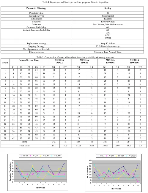
Figure 1 :Comparison of variable PI between Execution time and No. Test Cases
0 5 10 15 20 25 30 35 40
1 2 3 4 5 6 7 8 9 10
No. of Cases
N
o
.o
f
It
e
r
a
ti
o
n
PI=0.1 PI=0.01 PI=0.001 PI=0.0001
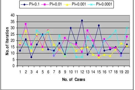
Figure 2 : Comparison of variable PI between No. of iteration and No. Test Cases
Parameter / Strategy Setting
Population Size 20
Population Type Generational
Initialization Random
Selection Roulette wheel
Crossover Two Parents, Modified crossover
Crossover Probability 0.6
Variable Inversion Probability 0.1
0.01 0.001 0.0001
Replacement strategy Keep 80 % Best
Stopping Strategy 85 % Population converge
No. of process to be Schedule 5
IV. EXPERIMENTAL SETUP
The Individual solutions are randomly generated to form an initial population. Successive generations of reproduction and crossover produce increasing numbers of individuals . Modified crossover operator with crossover probability Pc is 0.6 is taken. This operator is suitable for permutation coding. Crossover operator exploited the population or you can say that it can diversify the population. But due to the genetic drift some time the population is converge to the local optimal point, At that time crossover operation can not diversify the population. The inversion operator is explorative in nature ,it diversify the population ,but in general the probability of inversion is very low . so in our simulation We first have 0.1 inversion probability then we proceed with .01,.001.0001. The parameter setting for proposed genetic algorithm is as shown in table no .1.
0 5 10 15 20 25 30 35 40
1 2 3 4 5 6 7 8 9 10 11 12 13 14 15 16 17 18 19 20
No. of Cases
N
o
.o
f
It
e
r
a
ti
o
n
[image:5.612.68.291.209.358.2]PI=0.1 PI=0.01 PI=0.001 PI=0.0001
Figure 3 : Comparison of variable PI between No. of Iteration and No. Test Cases
0 1 2 3 4 5 6 7 8 9
1 2 3 4 5 6 7 8 9 10 11 12 13 14 15 16 17 18 19 20 No. of Cases
E
x
e
c
u
ti
o
n
T
im
e
i
n
S
e
c
.
[image:5.612.69.291.396.538.2]PI=0.1 PI=0.01 PI=0.001 PI=0.0001
Figure 4 : Comparison of variable PI between Execution time and No. Test Cases
V. EXPERIMENTAL RESULTS
In this experiment we have two slots of test cases i.e of 10 test cases and 20 test cases. Here modified crossover genetic algorithm is implemented to check the result . In the table no. 1 & 2 N.I. denote the no. of iteration , E.T. is execution time and P.I. is the probability of inversion .The experiment result shows that with PI =0.1 will reduce the no. of iteration and PI=0.0001 increase the no. of iteration.
VI. CONCLUSION
In this paper, we examine the effect of varying inversion probability on the performance of the genetic algorithm. when the inversion probability is very high then we can see with the result that population is pre converge to the local sub optimal point and when the probability is very low i.e. 0.0001 then the speed of the genetic algorithm is degraded . so we examine that inversion probability should be as much as that we will get optimal solution . Also we examine that the inversion probability should neither too low nor to high. It should be moderate i.e .001 is desirable. So by having appropriate inversion probability the performance of genetic algorithm can be Enhance to process scheduling problem
VI. REFERENCES
[1] K.R. Baker, (1974). Introduction to sequencing and scheduling, Wiley, New York.
[2] S. French, (1982). Sequencing and Scheduling: And introduction to the Mathematics of the Job Shop, Ellis Horwood, Chichester.
[3] M. Pinedo,, (2001), Scheduling – Theory, Algorithms and Systems, 2ª edição, Prentice-Hall.
[4] Brucker, P. (2001). Scheduling Algorithms, Springer, 3rd edition, New York.
[5] Holland, J.H., 1975. “Adaptations in natural and artificial systems”, Ann Arbor: The University of Michigan Press [6] M.Srininivas and L.M.Patnaik,”Genetic Algorithms: A
survey”, IEEE computer Magazine,pp.17-26,june 1994 [7] R.Kumar,(2010),”Genetic algorithm approach to operating
system process scheduling problem”,International journal of Engineering science and Technology,pp 4248-4253
[8] L.Davis. Job-shop scheduling with genetic algorithms.Van Nostrand Reinhold,1990