GNA: new framework for statistical data analysis
Anna Fatkina1, Maxim Gonchar1,∗, Anastasia Kalitkina1, Liudmila Kolupaeva1, DmitryNaumov1,DmitrySelivanov1, andKonstantinTreskov1
1Joint Institute for Nuclear Research, Dubna, Moscow, Russia
Abstract.We report on the status of GNA — a new framework for fitting large-scale physical models. GNA utilizes the data flow concept within which a model is represented by a directed acyclic graph. Each node is an operation on an array (matrix multiplication, derivative or cross section calculation, etc). The frame-work enables the user to create flexible and efficient large-scale lazily evaluated
models, handle large numbers of parameters, propagate parameters’ uncertain-ties while taking into account possible correlations between them, fit models, and perform statistical analysis.
The main goal of the paper is to give an overview of the main concepts and methods as well as reasons behind their design. Detailed technical information is to be published in further works.
1 Introduction
1.1 Interpretation of observables
The measurement of physical parameters from experimental data significantly relies on meth-ods of statistical inference. The main methmeth-ods of performing parameter inference are either maximum-likelihood-based (ML) or Bayesian. These approaches involve massive numerical computations when working with models with a large number of parameters, either free or constrained.
Searching for evidence of weak signals or having a limited sample of data often requires special numerical procedures to derive confidence intervals for parameters of interest. Ex-amples of such approaches are Feldman-Cousins (FC) [1] (pure frequentist) and Cousins-Highland [2] (hybrid Bayesian-frequentist) methods. The guarantee of correct coverage pro-vided by these techniques comes at the cost of extensive numerical computations, e.g. fitting a model to a large number of pseudo-experiments to derive the test statistic distribution.
Both signal weakness and finiteness of the data sample are common situations in modern neutrino physics. Searches for a light sterile neutrino in Daya Bay [3] and oscillation analysis of NOvA [4] are two examples among many of this kind, that use methods requiring high performance computing.
Performing high load statistical analysis with large-scale models requires dedicated soft-ware. Extra attention should be paid to long-term analysis consistency since the typical life-time of a modern neutrino physics experiment may achieve dozens of years.
1.2 Software
The most common tool to perform statistical data analysis used in high energy physics is currently ROOT [5] with the RooFit package [6] built on top of it. These tools are well-suited for inference and parameter estimation for relatively low-dimension problems with small numbers of model parameters. When the number of parameters in the analysis grows these tools become less flexible and efficient.
A new generation of software frameworks taking advantage of modern hardware and suitable for contemporary analysis needs is required. A few solutions are already available.
GooFit [7] is a library designed to perform maximum-likelihood fits in a fashion similar to RooFit but taking advantage of massive parallel computations with GPUs and modern CPUs through NVIDIA Thrust and OpenMP. It is used extensively in LHCb analyses [8].
Hydra [9] is a header-only library for statistical data analysis utilizing CUDA, OpenMP and TBB as backends. It offers maximum-likelihood fitting, tools for working with multidi-mensional PDFs, multidimultidi-mensional numerical integration with MCMC, and other tools.
Both of these libraries require model specification at compile time, which limits flexibility when working with varying models.
2 GNA
2.1 Design principles
Below we will list the typical analysis context and the features the user requires from the framework.
First of all we are aiming at large-scale models, such as Daya Bay model (variant D) [10], that may yield several histograms with hundreds of bins, contain thousands of elements and depend on hundreds of model parameters, some of them may be partially correlated. The parameters do affect various parts of the model and may be varied one-by-one, group-by-group, or all together. The common tasks done with a model include:
• computation of the derivative over a parameter,
• multidimensional ML fit with few parameters or with with hundreds of parameters, • 2d scan over two parameters with fit of all the remaining parameters in each point, • numerous fits to MC data, e.g. hundreds of thousands of fits within FC method [1], • combined study of a few models taking into account correlations between their parameters.
During the analysis preparation various parts of the model may be replaced by alternative parametrizations or approximations. Even the computation scheme itself may be significantly refactored. After the analysis results are published the model is maintained for a period of 5 to 10 years by different people with different experience in software development. Each analysis update may again require a significant model update while the subsequent analyses should be consistent with each other and the old analyses should be reproducible.
Based on this, the requirements to the framework include high flexibility, computational efficiency, expressiveness, easy maintainability and long-term backwards compatibility.
We are solving these issues by using the data flow paradigm [11]. The model is build at runtime as a directed acyclic graph. Each node represent an operation on an input data array(s) producing several output data arrays. The framework provides a library of precom-piled operations, also called transformations, that are required for the statistical analysis of physical data. The model is then assembled by binding instances of transformations together. This enables the user to concentrate on the logic and physics of the analysis while ignoring
the low-level issues, such as memory allocation. All of the internals are organized, acces-sible and reviewable. Computational graphs (chains) of different models may be combined together.
The transformations and transformation bundles are designed to be immutable. Instead of modifying the transformation it is suggested to extend the library by writing another one, which facilitates backwards compatibility.
The computational chain, maintained by GNA, is in fact a runtime call graph. This facili-tates the implementation, implicit from the user’s point of view, of powerful features, such as CPU multithreading, GPU support, etc.
There are a lot of parallels and similarities with the TensorFlow package [12] as well as some other data flow tools for neural networks. In fact, we are trying to simplify similar software tasks within a scope of statistical analysis of large scale physical models.
2.2 GNA core
GNA is implemented in C++and Python. The core is implemented in C++to provide ef-ficiency while the management code is written in Python to provide flexibility. GNA de-pends on the Eigen [13] library for array operations and ROOT package [5] responsible for minimization and C++/Python binding. Other dependencies include boost [14], GSL [15], numpy/scipy [16] and matplotlib [17].
The model in GNA is represented by a computational graph, that consists of nodes (Transformation) and edges connecting transformations’ outputs (Sink) to another trans-formations’ inputs (Source). The data arrays are allocated within transformation sinks. The sources, in contrast, hold no data: the source is a view to another transformation sink.
There are two templates for data types in GNA, variableand Data.variable is a wrapper for an elementary data type, usually double. Variables represent model parameters and may be used in a process of minimization, or derivative calculation, etc.
The Data is an array data type that ‘flows’ within a graph. It is allocated on transfor-mations’ sinks and holds a buffer. TheData is characterized by aDescriptor that holds the information on size, dimension and type of the data.Datamay be a regular array or a histogram. In the latter case theDescriptoralso carries an array of bin edges.
Variables and transformations carrytaintflagthat indicates the validity of the stored data. The flags are connected in a graph. Whenever a variable is modified it becomes tainted. The taint flag is then propagated to all the dependent objects, variables and transformations, invalidating a part of the computational graph. When the output of the untainted mation is accessed the cached result is returned. If the transformation is tainted the transfor-mation function is called in order to update the data. The function itself may read the other transformations’ data triggering a chain of updates. Finally, only the part of the graph that is tainted and that is required to build the requested data is executed, other parts either return cached data or are not touched at all. This effectively implements lazy evaluation of a graph.
2.3 GNA usage
The transformation is defined by several C++functions: one for calculation and a few for type checking. The calculation function may access transformation sources and sinks and is used to compute the result. It is executed if the output of tainted transformation is accessed.
case of a transformation implementing matrix multiplication the user binds two matrices to the transformation sources:N×MandM×K. When inputs are bound, the transformation’s first type function will check that the matrices are indeed multipliable or throw an exception otherwise. The second type function will tell that the output should have dimensionsN×K and the framework will allocate the relevant array at the only transformation sink.
Thus, the two stages may be outlined in GNA model usage: the binding stage and calcu-lation stage. At the first stage, when the transformations are being instantiated and bound, the framework derives data types and allocates memory. The variables are bound to the transfor-mations on the first stage as well. While the first stage may not be that efficient it is typically executed only once. At the second stage the model is repeatedly used for computation. Since the framework guarantees that the inputs and outputs passed to the computation functions are of proper shape the corresponding checks are omitted in the computation functions, which makes them more readable and efficient.
A special remark should be made on the integration process. The GNA work flow implies that the transformations operate on arrays and that at the calculation stage the computational graph has all the required memory allocated. In such a deterministic scheme the integration process should also be explicitly vectorized, which also means that the integration precision is chosen beforehand. Since GNA is aimed at fitting models to data we assume that in most cases the integration precision may indeed be defined in prior.
The integration process is then split into two transformations. For a given set of bin edges xiand integration ordersMithe first transformation samples all the pointspi jand weightsωi j
needed to compute the integral for each bin. The set of pointspi jis then passed to a function
of interest1as an array. The second transformation then convolves the output of the function f(pi j) with provided weights, producing a histogram. The 1D case reads as follows:
Hi=
xi+1
xi
f(x)dx≈
Mi
ji=1
ωi jf(pi j). (1)
The weights and points are computed once. The method of Gauss-Legendre (GL) quadratures is implemented in GNA for 1 and 2 dimensions with an easy extension to other methods.
A similar deterministic approach is applied to spline interpolation. Since the target points are known beforehand the binary search is extracted to a separate transformation which is executed only once. One of the benefits of the approach is that it enables effective usage of the framework’s caching nature. For example, in the following integral σ(E)P(E)S(E)dE the computationally expensive cross sectionσ(E) might not depend on varying model parameters and will be evaluated only once at runtime, while the computationally cheaper probability P(E) and spectrum shapeS(E) depend on the minimization parameters and will be evaluated on each execution, following the variation of relevant parameters.
2.4 Transformations, bundles and expressions
The GNA framework provides a library of transformations required for building models and performing statistical analysis of data. Some of the included transformations are basic opera-tions (sum, product), linear algebra (Cholesky decomposition), statistics (χ2, covariance ma-trix and Poisson log-likelihood calculation), calculus (differentiation and integration), physics (neutrino oscillations probability, inverse beta decay cross section), and detector effects (en-ergy smearing, en(en-ergy response distortion). There is a focus on reactor neutrino physics due to the fact that the project has grown from the analysis of Daya Bay experimental data.
1the function may be represented by a single transformation or a small computational chain.
Even after the transformations are introduced, combining them may be quite a tedious job. To make it easier we introduce bundles and expressions. ABundleis a Python class that reads a dictionary containing the configuration and initializes a set of variables and instantiates and binds a set of transformations. The result ofBundleexecution is a small computational chain. A special tool is provided for the purpose of binding small computational graphs together to form a large chain. The concept calledExpressionis using mathematical expressions to describe connections between transformations and bundles.Expressionis initialized with the following information: a) a mathematical expression, b) the definition of indices used in the expression, c) configurations for the bundles to be executed to provide expression elements.
The expressions are parsed within a predefined python environment and are valid python expressions. The only distinction is that we are using the’func| arg1, arg2, ...’ no-tation for’func(arg1, arg2, ...)’in order to improve the readability of the chain calls. Consider the following example:
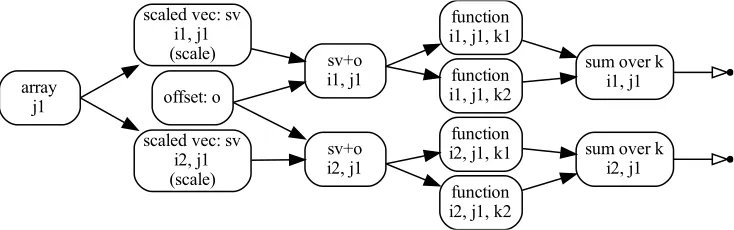
sum[k]| func[k]| scale[i] * vec[j]() + offset() (2) The expressions are parsed without actual knowledge of what data and functions are: each name is considered to be an index, variable or transformation output. Herevec[j]()is a transformation output providing an array. The bundle that will providevecwill provide an output for each variant of indexj.scale[k]is a variable with variants fork1,k2, etc. The multiplicationscale[i] * vec[j]()will provide a transformation that scales an array for each combination of indices ofiandj. Then theoffsetarray will be added to each result.
funcis a function with one argument and one return value. The call operation means that the output, associated with the argument, is bound to the input, associated with a function. As in the case of multiplication each permutation of indices is taken into account. Since there is an output for each combination ofi andj values and functions have several variants, represented by indexk, a call will produce an output for each permutation of i,j andk variants. Lastly thesum[k]will make a sum over indexkand provide the output for each of iandjvariants. Then, for each unknown name theExpressionfinds a bundle configuration and executes the corresponding bundle, passing the indices assigned to the name. The bundle should then provide all the necessary inputs, outputs and variables. Once bundles are executed Expressionwill bind the transformations together.
The result of the expression (2) for the case when indexihas variants{i1,i2},j∈ {j1} andk ∈ {k1,k2}is shown in figure 1. The graph represents only transformations and their connections while variables are not plotted.
offset: o sv+o i1, j1 sv+o i2, j1 function i1, j1, k1 function i1, j1, k2 function i2, j1, k1 function i2, j1, k2
sum over k i1, j1 scaled vec: sv
i1, j1 (scale) array
j1
scaled vec: sv i2, j1 (scale)
sum over k i2, j1
Figure 1.An example of the computational chain, produced by expression (2).
a set of bundles, is enough to build large-scale models. For example, the Daya Bay model is described by 6 indices, roughly 50 items in the expression, 25 configuration items that are using 16 bundles. TheExpressionproduces a computational chain of 732 nodes and 1624 edges (736 outputs with 13.6 Mb of data); 498 parameters (114 fixed, 97 variable and 287 evaluated). The full computational time is 10 ms. Only a slight modification of the order of instructions in the expression yield a very different computational graph with 2412 nodes and 5968 edges (4416 outputs with 20.3 Mb of data). The latter chain produces identical result with a full computational time of 20 ms. A more detailed description of the example may be found in [18].
3 Prospects
Since GNA has full control over how the computational chain is executed it is possible to introduce alternative mechanisms utilizing modern computation techniques on a level of the framework, i.e. implicitly for the end user. Our development team is working on GPU and multithreading support in order to make GNA suitable for heterogeneous systems. In the following chapter an overview of the task manager for multicore CPU and GPU support is given.
3.1 Multithreading
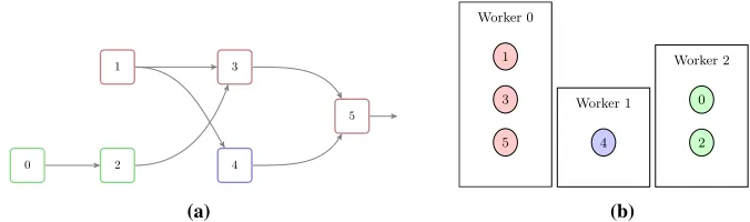
Different parts of the GNA computational graph may be executed in parallel threads with each transformation representing a task. Due to the lazy and caching nature of GNA the evaluation order is not fixed and depends on the computational chain state and the transformation which the output is called. The multithreading support was introduced in order to manage execution and assign tasks to workers at runtime.
A thread pool is implemented with workers assigned to parallel threads. When the trans-formation output is called the support system traverses the computational graph and pushes the tainted transformations into workers’ stacks as distinct tasks. The first subsequent trans-formation is pushed into the current thread worker’s stack. The other transtrans-formations are pushed into either new workers’ stacks or free workers’ stacks. In case the task is accessing the transformation which is being computed in another thread the reading is blocked until the computation is finished.
1 3
5
0 2 4
(a)
Worker 0 Worker 0
5 3 1
Worker 1 Worker 1
4
Worker 2 Worker 2
2 0
(b)
Figure 2.Task management scheme for the case of three threads. Example graph is shown
in (a) with colors representing the worker. Workers’ stacks are shown in (b) for the case when the output of 5th transformation is called.
a set of bundles, is enough to build large-scale models. For example, the Daya Bay model is described by 6 indices, roughly 50 items in the expression, 25 configuration items that are using 16 bundles. TheExpressionproduces a computational chain of 732 nodes and 1624 edges (736 outputs with 13.6 Mb of data); 498 parameters (114 fixed, 97 variable and 287 evaluated). The full computational time is 10 ms. Only a slight modification of the order of instructions in the expression yield a very different computational graph with 2412 nodes and 5968 edges (4416 outputs with 20.3 Mb of data). The latter chain produces identical result with a full computational time of 20 ms. A more detailed description of the example may be found in [18].
3 Prospects
Since GNA has full control over how the computational chain is executed it is possible to introduce alternative mechanisms utilizing modern computation techniques on a level of the framework, i.e. implicitly for the end user. Our development team is working on GPU and multithreading support in order to make GNA suitable for heterogeneous systems. In the following chapter an overview of the task manager for multicore CPU and GPU support is given.
3.1 Multithreading
Different parts of the GNA computational graph may be executed in parallel threads with each transformation representing a task. Due to the lazy and caching nature of GNA the evaluation order is not fixed and depends on the computational chain state and the transformation which the output is called. The multithreading support was introduced in order to manage execution and assign tasks to workers at runtime.
A thread pool is implemented with workers assigned to parallel threads. When the trans-formation output is called the support system traverses the computational graph and pushes the tainted transformations into workers’ stacks as distinct tasks. The first subsequent trans-formation is pushed into the current thread worker’s stack. The other transtrans-formations are pushed into either new workers’ stacks or free workers’ stacks. In case the task is accessing the transformation which is being computed in another thread the reading is blocked until the computation is finished.
1 3
5
0 2 4
(a)
Worker 0 Worker 0
5 3 1
Worker 1 Worker 1
4
Worker 2 Worker 2
2 0
(b)
Figure 2.Task management scheme for the case of three threads. Example graph is shown
in (a) with colors representing the worker. Workers’ stacks are shown in (b) for the case when the output of 5th transformation is called.
There exist various strategies on how to assign tasks to workers. We have chosen the ‘wide’ strategy that tries to execute maximally independent branches in parallel threads. An example scheme of the runtime task management for 3 threads is shown in figure 2. When the output of transformation 5 (T5) is read it is pushed to the worker 0 (W0),T3is then pushed
to the same worker andT4to the new workerW1. On the next step the inputs ofT3 andT4 are considered:T1is pushed toW0(same worker withT3),T2to the new workerW2.T4then will wait for theT1to be finished byW0.T0is added toW2.
Due to the fact that transformations, which access the same outputs from parallel threads, are temporarily blocked the efficiency of such an approach to multithreading will be below 100% and will depend on the computational chain structure. The actual efficiency will be studied in the future.
3.2 GPU
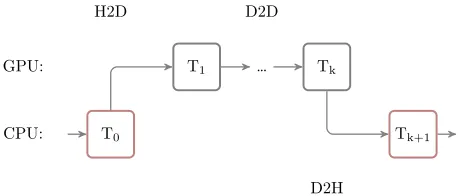
GPU support through CUDA [19, 20] for GNA was recently announced in [21]. Preliminary test results were presented showing x20 speed up of neutrino oscillation probability calcula-tions when compared to the single-core CPU version. We used a laptop powered by NVIDIA GTX 970M and Intel Core i7-6700HQ. These tests were done with double precision floating-point operations since, at the moment, this is the only precision supported by the framework. GNA provides great flexibility due to the fact that individual transformations, while being compiled independently from each other, may be combined at runtime into any computational scheme. The GPU support follows a similar paradigm. Unified interfaces are introduced to provide GPU-based implementations of the transformations in a similar way as CPU-versions are done. The transformation may be switched between CPU and GPU implementations at runtime. GPU memory is allocated when required and implicit data transfers between CPU and GPU occur lazily at runtime.
The computational chain example with GPU transformations involved is shown in fig-ure 3. A series of GPU based transformations T1 toTk are situated between CPU based
transformationsT0andTk+1. A memory transfer from host to device (H2D) is invoked when aT1 transformation is called, a transfer back from device to host (D2H) is triggered only when CPU basedTk+1reads the output of GPU basedTk. It is essential that no data transfer between host and device is invoked between consequential GPU transformations.
H2D D2D
GPU: T1 … Tk
CPU: T0 Tk+1
D2H
Figure 3.An example of hybrid CPU/GPU graph.
It is also worth noting that typical GPUs provide superior efficiency for single precision floats when compared to double precision. A way to choose the computational chain precision will be provided so that the user can check the model performance and switch to single precision.
Further prospects of combined CPU/GPU usage are also considered. They include the hybrid case when different GPU transformations are invoked from parallel threads. In the massively parallel case several dozens of replicas of the same model may be merged and executed on GPU in a single call. Therefore the maximal profit may be achieved in a case when these models are used for parallel fitting to different MC samples or different points of a studied parameter space.
4 Conclusion
We present an overview of methods implemented in GNA, a framework for statistical analysis of large-scale models. GNA uses the data flow paradigm to provide a way to build caching and efficient lazily evaluated models. The models may be assembled at runtime, thus giving the user high flexibility. There are inspiring prospects to include, implicitly from the end user point of view, multithreading on CPU and GPU support.
The framework is currently under active development with many features introduced re-cently. As long as the code base is not yet finalized the development is carried out in a private repository. After finalizing and cross checking the Daya Bay [18] model, we will suspend the active development phase in order to prepare a production release. We plan to review and document the GNA framework in early 2019 and make the project public by Spring 2019.
The current project page may be found in [22]. The documentation page [23] is slightly outdated while the reference guide section [24] contains an actual description of the subset of transformations and tools.
Acknowledgements
The research is supported by the Russian Foundation for Basic Research (grant 18-32-00935) and by Association of Young Scientists and Specialists of JINR (grant 18-202-08).
We are grateful to Chris Kullenberg for reading the manuscript and for the valuable com-ments.
References
[1] G.J. Feldman, R.D. Cousins, Phys.Rev.D57, 3873 (1998),physics/9711021 [2] R.D. Cousins, V.L. Highland, Nucl. Instrum. Meth.A320, 331 (1992)
[3] F.P. An et al. (Daya Bay), Phys. Rev. Lett.117, 151802 (2016),1607.01174 [4] P. Adamson et al. (NOvA), Phys. Rev. Lett.116, 151806 (2016),1601.05022 [5] R. Brun, F. Rademakers, Nucl.Instrum.Meth.A389, 81 (1997)
[6] W. Verkerke, D.P. Kirkby, eConfC0303241, MOLT007 (2003), [,186(2003)] [7] R. Andreassen et al., J. Phys. Conf. Ser.513, 052003 (2014),1311.1753 [8] R. Aaij et al. (LHCb), Phys. Rev.D93, 052018 (2016),1509.06628
[9] A.A. Alves Junior (2018), (visited on 2019-02-22), https://doi.org/10.5281/ zenodo.1206261
[10] F.P. An et al. (Daya Bay), Phys. Rev.D95, 072006 (2017),1610.04802
[11] J.B. Dennis, J.B. Fosseen, J.P. Linderman, Data flow schemas (Berlin, Heidelberg, 1974), pp. 187–216, ISBN 978-3-540-38012-2
[12] M. Abadi et al.,TensorFlow: Large-scale machine learning on heterogeneous systems (2015), (visited on 2019-02-22),http://tensorflow.org
[13] G. Guennebaud, B. Jacob et al.,Eigen v3, http://eigen.tuxfamily.org (2010), (visited on 2019-02-22)
[14] boost C++libraries, (visited on 2019-02-22),https://www.boost.org
[15] M. Galassi, J. Davies, J. Theiler, B. Gough, G. Jungman,GNU Scientific Library - Refer-ence Manual, Third Edition, for GSL Version 1.12 (3. ed.)(Network Theory Ltd, 2009), ISBN 978-0-9546120-7-8, (visited on 2019-02-22),http://www.network-theory. co.uk/gsl/manual/
[16] E. Jones et al. (2001), (visited on 2019-02-22),http://www.scipy.org/ [17] J.D. Hunter, Computing in Science & Engineering9, 90 (2007)
[18] A. Fatkina, M. Gonchar, D. Naumov, K. Treskov (2018), collaboration meeting talk (vis-ited on 2019-02-22), https://astronu.jinr.ru/wiki/images/7/75/2018.10_ dayabay_gna.pdf
[19] NVIDIA,Compute unified device architecture (CUDA) programming guide(2007) [20] J. Nickolls, I. Buck, M. Garland, K. Skadron, Queue6, 40 (2008)
[21] A. Fatkina et al.,CUDA Support in GNA Data Analysis Framework(2018), pp. 12–24 [22] GNA home page, (visited on 2019-02-22), https://astronu.jinr.ru/wiki/
index.php/GNA
[23] GNA documentation, (visited on 2019-02-22),http://gna.pages.jinr.ru/gna/ [24] GNA reference guide, (visited on 2019-02-22), http://gna.pages.jinr.ru/gna/