The Prohorov Metric Framework and Aggregate
Data Inverse Problems for Random PDEs
H. T. Banks
1, K. B. Flores
1, I. G. Rosen
2, E. M. Rutter
1,
Melike Sirlanci
2, W. Clayton Thompson
1,3June 13, 2018
1Center for Research in Scientific Computation
Department of Mathematics North Carolina State University
Raleigh, NC and
2Department of Mathematics
University of Southern California Los Angeles, CA
and
3SAS Institute
Cary, NC
Abstract
We consider nonparametric estimation of probability measures for pa-rameters in problems where only aggregate (population level) data are available. We summarize an existing computational method for the esti-mation problem which has been developed over the past several decades [24, 5, 12, 28, 16]. Theoretical results are presented which establish the existence and consistency of very general (ordinary, generalized and other) least squares estimates and estimators for the measure estimation problem with specific application to random PDEs.
Key Words: Inverse problems, aggregate data, individual data, existence and approximation of estimators.
1
Introduction
Our ideas of using distributions for parameters in inverse problems grew out of work in [7] and use of Sinko-Streifer models for mosquitofish growth rates where only aggregate data were available due to periodic sampling of different subsets of the population. The first theoretical results in the context of inverse problems was in [12]. There were numerous subsequent uses including shrimp population size models in [4, 11] and carboxyfluorescein succinimidyl ester (CFSE) label-ing models [13]. In our presentation here we consider approximation methods in estimation or inverse problems but the quantity of interest is a probability distribution. Assume we have a parameterized system (q∈Ω) with state model responsesx(t;q) describing the population of interest. For data or observations, we are given a set of values{yl≈Cx(tl;q)}for the expected values
E[yl(q)|P] =
Z
Ω
yl(q)dP(q)
for observationsyl(q) =Cx(tl, q) with respect to the unknown probability
dis-tributionP describing the distribution of parameters qover the population. We use data to choose from a given family of distributions P(Q) the dis-tribution P∗ that gives the best fit of the underlying model to data. This is
accomplished by formulating an ordinary least squares (OLS) problem; how-ever we note that we could equally well use a weighted least squares (WLS) or maximum likelihood estimation (MLE) framework. Specifically we seek to minimize
J(P) =X
l
|E[yl(q)|P]−yl|2
over P ∈ P(Ω). Even for simple dynamics for yl(q) this yields an infinite
dimensional optimization problem. Therefore one needs approximations that lead to computationally tractable schemes. That is, it is useful to formulate methods to yield finite dimensional setsPM(Ω) over which to minimizeJ(P).
Of course, we wish to choose these methods so that “PM(Ω) → P(Ω)” in
The data{yl} available (which, in general, will involve longitudinal or time
evolution data) determines the nature of the problem. In gerneral there are three classes of problems:
• Type I: The most classical problem (which we shall refer to as aType I
problem) is one in which individual longitudinal data is available for each member in the population. In this case there is a wide statistical literature (in the context of hierarchical modeling, mixing distributions, mixed or random effects, mixture models, etc.) [29, 33, 34, 35, 36, 50, 49, 51, 53, 65, 64, 63] which provides theory and methodology for estimating not only individual parameters but also population level parameters and allows one to investigate both intra-individual and inter-individual variability in the population and data.
• Type II: In what we shall refer to asType IIproblems one has only ag-gregateor population level longitudinal data available. This is common in marine, insect, etc.,catch and releaseexperiments [17] where one samples at different times from the same population but cannot be guaranteed of observing the same subset of individuals at each sample time under con-stant environmental, etc., conditions. This type of data is also typical in experiments where the organism or population member being studied is sacrificed in the process of making a single observation (e.g., certain phys-iologically based pharmacokinetic (PBPK) modeling [1, 21, 66, 57] and whole organism transport models [17]). In this case one may still have dynamic (i.e., time course) models for individuals, but no individual data are available.
• Type III: Finally, the third class of problems which we shall refer to as
Type IIIproblems involves dynamics which depend explicitly on the prob-ability distributionP itself. In this case one only has dynamics (aggregate dynamics) for the expected value
¯
x(t) =E[x(t, q, P)|P]
of the state variable. No dynamics are available for individual trajectories
While the approximations we discuss below are applicable to all three types of problems, our primary interest here is problems of Type II and Type III. In particular we shall illustrate and provide theoretical underpinnings for our ear-lier computational results in the context ofTransdermal Alcohol Concentration (TAC) and Glioblastoma Multiforme (GBM) cancer where the inverse prob-lems are of Type II. Finally, we note that in the probprob-lems considered here, one
can not sample directly from the probability distributionbeing estimated and this again is somewhat different from the usual case treated in some of the statistical literature, e.g., see [81, 82] and the references cited therein.
2
Example 1: Estimating Blood/Breath
Alco-hol Concentration from Transdermal AlcoAlco-hol
Concentration(TAC)
The measurement of the alcohol level in the human body for the purpose of med-ical research, clinmed-ical therapy, and law enforcement (e.g. DUI, etc.), typmed-ically takes the form of blood alcohol concentration (BAC). However, in the absence of a blood sample, which is almost always the case, a surrogate, breath alcohol con-centration (BrAC) as measured by an instrument known as a breath analyzer, is used. The underlying chemistry of the breath analyzer (based on Henry’s Law [48]) has been shown to be reasonably robust and consistent across individuals and ambient conditions, thus allowing for the relatively straight forward con-version of breath alcohol concentration (BrAC) to blood alcohol concentration (BAC). Unfortunately, however, there are two significant drawbacks to collect-ing data uscollect-ing a breath analyzer: properly blowcollect-ing into a breath analyzer so as to obtain accurate measurements can be challenging, and the collection of breath data that is near-continuous in time and in a naturalistic setting is all but impossible.
Recently, technology has been developed to allow for the measurement of transdermal alcohol, or alcohol that diffuses from the skin’s dermal layer which has an active blood supply, through the epidermal layer of the skin. These devices use a variety of technologies (electro-chemical, enzymatic, optical, etc.) to count the number of ethanol molecules evaporating from the surface of the skin through normal perspiration. The current generation of transdermal alco-hol biosensors are reasonably compact and relatively unobtrusive, and generally resemble a digital watch, ankle bracelet, or activity tracker. Two such devices are the WrisTASTM7 alcohol biosensor designed and manufactured by Giner, Inc. of Waltham, MA and the Secure Continuous Alcohol Monitoring System (SCRAM) device manufactured by Alcohol Monitoring Systems in Littleton, Colorado (see Figure 1). These devices offer the possibility of passively
collect-Figure 1: Alcohol Biosensor Devices: The WrisTAS (left) and the SCRAM (right).
that is essentially continuous in time over extended periods such as hours, days, or even weeks. It is also conceivable that they could be further miniaturized and included as a feature in the next generation of wearable health monitoring tech-nology. At present, however, with the exception of one company that monitors abstinence of DUI offenders under contract to the courts, these devices are pri-marily only being used in the research community, with the devices themselves (their utility, practicality, accuracy, dependability, etc.) the central focus of the research project. This is because while it has been known for a long time that the alcohol level in perspiration correlates well with the alcohol concentration in the blood or breath [77, 78, 79, 80], there are significant variations (1) from sen-sor to sensen-sor and (2) in the rate at which alcohol diffuses through the skin both across individuals and across distinct drinking episodes within individuals under differing environmental conditions. Consequently the meaningful quantitative interpretation of transdermal alcohol levels poses a significant challenge. More to the point, there is currently no known direct and generally accepted method for converting what these devices measure, transdermal alcohol concentration or TAC, to the quantities that researchers, clinicians, law enforcement and the public at large are all most familiar with and that are well understood measures of intoxication, BAC and/or BrAC.
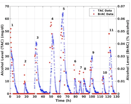
Some of the difficulties involved in converting TAC to BAC or BrAC are il-lustrated in the following two example data sets. A WrisTASTM7 was worn by a participant for 18 days. During each drinking episode, the participant collected BrAC data (i.e., blew into a breath analyzer) approximately every 30 minutes. The first drinking episode was conducted in the laboratory and BrAC was mea-sured every 15 minutes until it returned to 0.000. The participant then wore the device for the following 17 days and consumed alcohol ad libitum. During those days, BrAC was measured every 30 minutes starting from the beginning of the drinking session until its value returned to 0.000. The WrisTASTM7 measured and recorded ethanol level at the skin surface every 5-minutes. During those 17 days, the data were collected in a naturalistic setting. The plot in Figure 2 shows the measured BrAC and TAC over 11 drinking episodes. Note that in drinking episodes 1, 2, 4, 6, 7, 8, and 11 the peak BrAC value was higher than the bench calibrated peak TAC value, while in drinking episodes 3, 5, 9, and 10 the peak TAC value was higher than the peak BrAC value.
Figure 2: BrAC and TAC measurements for multiple drinking episodes by a single subject.
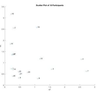
observed TAC, as the scatter plot below clearly shows, there was nevertheless a wide variance in the values of the fit parameters.
Figure 3: Scatter plot of deterministically obtained parameter estimates for BrAC and TAC measurements from a single drinking episode from each of 18 subjects.
disorder).
In a more recent series of papers [69, 67, 70], this same research group has proposed eliminating the need to calibrate the forward models, by developing population models based on their physics based models. The parameters in the model are assumed to be random and instead of using their actual values as a basis for fitting the model, the training data is used to estimate the distribution of these random parameters. In those studies, however, the arguments used to demonstrate the convergence of their method required the assumption that the distributions were described by appropriately constrained parameterized fami-lies of probability density functions. The theory we describe here demonstrates how this restrictive assumption can be eliminated.
By essentially converting all quantities in our first principles physics based model to dimensionless variables, we are able to eliminate some non-identifiable (i.e., dependent) parameters and obtain the initial-boundary value problem given by
∂ϕ
∂t(t, η) =q1 ∂2ϕ
∂η2(t, η), 0< η <1, t >0, (1)
q1
∂ϕ
∂η(t,0) =ϕ(t,0), t >0, (2) q1
∂ϕ
∂η(t,1) =q2u(t), t >0, (3) ϕ(0, η) =ϕ0, 0< η <1, (4)
trans-port of ethanol through the epidermal layer of the skin, and the boundary conditions (2) and (3) describe respectively the evaporation of ethanol at the skin surface (η = 0) and the flux of ethanol across the boundary between the epidermal and dermal layers of the skin (η = 1; note that the dermal layer has a blood supply whereas the epidermal layer does not). The initial conditions are given in (4) (typically we will haveϕ0= 0 since we will assume that at the
start of any drinking episode there is no alcohol in the body) and the output equation, (5) says that TAC is measured by the biosensor at the skin surface. The state of the system,ϕ(t, η) essentially denotes the concentration of ethanol at depthη,0 ≤η≤1 in the epidermal layer at timet≥0, whileu(t) andy(t) denote, respectively, the BAC/BrAC and TAC at time t. The parameters q1
(normalized “diffusion”) andq2 (normalized flux control input coefficient) are
assumed to lie in a compact subset, Q, of R+×R+ endowed with the metric
dQ.
While our ultimate goal is to deconvolve the BAC/BrAC input ufrom the biosensor measured TAC outputy, our concern in this study is dealing with the uncertainty in the model parameters. Indeed, since the parametersqwhich are unknown and dependent on 1) the individual wearing the sensor, 2) the ambient environmental conditions at the time the TAC measurements or observations were made, and 3) the particular sensor being worn, the problem of estimating BAC/BrAC from observations of TAC is in fact a blind deconvolution prob-lem involving aggregate data. Our approach involves replacing theq-dependent model with a population model which captures and quantifies the variability and uncertainty that exists across all the individual members of the population (we use the termindividualto mean not just different subjects, but alsounmodelled different environmental conditions and different hardware, and for that matter
any other un-modeled dynamics present in the system). Thus we view our prob-lem as the class of Type II described in the Introduction. The details involved in deconvolving the BAC/BrAC from the TAC once the population model has been estimated along with associated error bars can be found in [68].
We define thepopulation modelto be the system (1)-(5) with the parameters
q ∈ Q defined to be a random vector together with the distribution for the parameters in the form of a probability measureP0or joint distribution function
F0. We assume (1) thatν data sets (˜ui,y˜i)νi=1= {u˜i,j}νji=0−1,{y˜i,j}νj=0i ν
i=1 have
been collected, and (2) the statistical model given by ˜
Yi,j=E[Yj(q, ui)|P0] +Ei,j, j= 0, ..., νi, i= 1, ..., ν, (6)
where in (6), Yj(q, ui) is the random variable corresponding to (1)-(5) and
Ei,j, j= 0, ..., νi, i= 1, ..., ν, represent measurement noise and are assumed to
be independent and identically distributed with mean 0 and common variance
σ2. Then forP a probability measure defined on theσ-algebra of events in the probability space associated with the random vectorq, andF its corresponding cumulative distribution function, define for an observation operator ˆC(q) the the mean behavior at timej,j= 0, ..., νi,
vi(j;P) =E[yj(q, ui)|P] =
R
whereq∼F andyj is a realization for Yj .
The estimation problem is then to estimate the measure P0, using a least
squares approach
ˆ
P0= argmin
P
J(P; (˜ui,y˜i)νi=1) = argmin
P ν
X
i=1
νi X
j=0
(˜yi,j−vi(j;P))2. (8)
3
Example 2: Glioblastoma Multiforme (GBM)
Glioblastoma Multiforme (GBM) is a deadly primary brain tumor. Due to it’s highly infiltrative nature, GBM remains difficult to treat: although resection surgery may remove the primary tumor, many tumor cells can remain through-out the brain, resulting in nearly all tumors recurring [83]. It has been shown that tumors that exhibit nodular growth patterns (i.e., low diffusivity) result in better patient prognosis [2]. Thus, it is increasingly important to be able to accurately ascertain the growth and diffusion phenotypes present in individual tumors.
GBM is often modeled in vivo using partial differential equations. The simplest models of GBM growth only consider the reaction-diffusion equation [55, 75, 61], given by:
∂c(t, x)
∂t =D
∂2c(t, x)
∂x2 +ρc(t, x)(1−c(t, x)) (9)
wherec(t, x) represents the cell density at timetand spatial locationx,Dis the diffusion coefficient, andρis the intrinsic growth rate. However, this simplistic model assumes diffusion is isotropic, which does not accurately describe resulting
in vivo tumor shapes.
There are multiple methods to incorporate anisotropic diffusion in order to make glioma models more physiologically accurate. These methods introduce heterogeneity into the diffusion coefficients. For example, one can incorporate a spatially-dependent piece-wise diffusion coefficient to explain diffusion of cells in grey matter versus white matter [76]. In a similar vein, diffusion weighted imaging (DWI), which contains information about water diffusion, has been used to infer cellular diffusion through the brain [30, 31, 46, 47, 56]. Other approaches to incorporating cellular heterogeneity include density-dependent diffusion functions [73].
A landmark study discovered that, evenin vitro, a reaction-diffusion equa-tion was insufficient to describe the cellular dynamics [71]. In the work, the au-thors performed cell line experiments on most common mutation of Epidermal Growth Factor Receptor gene (U87∆EGFR) and wild-type EGFR (U87WT). This showed there are distinct behavioral differences between ‘migrating’ cells and ‘proliferating cells’ and thus concluded that migrating and proliferating cells should be modeled separately. This observation resulted in the modeling of cellular heterogeneity as a collection of two phenotypic subpopulations, one of which mainly migrated and one that mainly proliferated. This “go or grow” hypothesis [45] remains widely used in mathematical models of glioma growth today [72, 43]. For a recent review on the status of mathematical modeling in GBM see [54].
frequent measurements of the changing populations, one expects (because of a continuum of growth/death of the individual cells) this to represent (as in the case of many biological cell data counts [13]) aggregates of different populations at different times of data collections.
In [60], we proposed a model of GBM growth with the option of phenotypic heterogeneity by using parameter distributions for the parametersρandD. The random differential equation for GBM growth and diffusion is given by:
∂c(t, x;DDD, ρρρ)
∂t =∇ ·(DDD∇c(t, x;DDD, ρρρ)) +ρρρc(t, x;DDD, ρρρ)(1−c(t, x;DDD, ρρρ)) (10)
whereDDD andρρρare random variables defined on a compact set Ω = ΩDDD×Ωρρρ.
In order to obtain the aggregate observable, we take the expectation over all subpopulations:
v(t, x) =E[c(t, x;·,·), P] =
Z
Ω
c(t, x;DDD, ρρρ)dP(DDD, ρρρ) (11)
The given random differential equation has the option of phenotypic heterogene-ity because we can easily recover the basic reaction-diffusion equation (Eq. 9) whenDDD andρρρare point distributions. Moreover, we are able to model a “go or grow” system by considering bigaussian distributions of the parameters. Most importantly, we are able to model these distributions (and more) without mak-ing any assumptions on the underlymak-ing distributions.
Several different methods for approximating the probability measuresP(DDD, ρρρ) include using either discrete approximations based ondelta functionsor continu-ous approximations based onspline basis functions. Although using higher order spline functions are known [3, 9, 10, 20] to yield more accurate convergence in the case of smooth probability density functions (PDF) and cumulative distri-bution functions (CDF), delta functions are able to better approximate CDFs that have discontinuous derivatives. Therefore, in [60] we discussed the use of both approximations since we did not wish to make any assumptions about, or restrictions on, the CDF.
Suppose that the aggregate spatiotemporal data we want to model is given byvji, representing the data at timejand spatial locationi, wherej= 1, .., Nt
andi= 1, ..., Nx. Then, we estimate usingN =Nt×Nxdata points
ˆ
PN = argmin P(Ω)
Nt,Nx X
j,i=1
(vji−v(tj, xi;P))2.
(This, of course, is an idealized version of available data sets but we will use this notation when discussing consistency. We assume in our subsequent discussions involvingN→ ∞statements it is understood bothNt, Nx→ ∞.)
This becomes
ˆ
PN = argmin P(Ω)
X
j,i
vji−
Z
Ω
c(tj, xi;DDD, ρρρ)dP(DDD, ρρρ)
2
(12)
4
Prohorov Estimates and Their Approximations
Convergence in the Prohorov metric is equivalent to the weak* convergence of measures when the space of probability measures P(Ω) is imbedded in the dual C∗(Ω) of the space of bounded continuous functions on Ω. We discuss briefly existence, convergence, and consistency theory, assuming here we are only estimatingDDD of the GBM example above as a distribution. We note the theory readily extends to two parameters (diffusion and growth rates) for the GBM example and to the vector parameters in the case of the TAC example discussed above.
In the following discussions we adopt the following notation :N = (Nt, Nx) =
Nt×Nxare the number of data points or observations;v
˜
N(t, x;ω) are the state
approximations tov(t, x;ω), so ˜N is the index for state approximations;M will be the parameter approximation index
We assume a familyP(Ω) of permissible probability functions for our diffu-sion rates. We attempt to perform the estimation in a least-squares framework
ˆ
PN = argmin P∈P(Ω)
JN(~v, P) = argmin P∈P(Ω)
N
X
j,i
(vji−v(tj, xi;P))2 (13)
where N observations are used to obtain a best fit for a nominal or “true” parameterP0. In order to approximate this minimizer, we replace the infinite
dimensional optimization problem by a sequence of finite-dimensional optimiza-tion problems with, for example, Dirac or spline-based distribuoptimiza-tions. Thus, if we use the Dirac approximating families, we setDDDM ={∆Dk, k= 1, .., M}, where
M represents the number of nodes, or elements, used in the approximation. Our family of approximating probability functions becomes
PM(Ω) =nPM = M
X
k=1
wk∆Dk|wk ≥0 and
M
X
k=1
wk = 1
o
,
where ∆Dk represents the Dirac delta function at the point Dk and wk are the
weights and/or probabilities. It has been previously proven [23, 28] that there exists a minimizer for the discrete approximation problem
ˆ
PNM = argmin
P∈PM(Ω)
Nt,Nx X
j,i=1
(vji−v(tj, xi;P))2. (14)
A further approximation arises when we appproximate the state variablev by numerical approximationvN˜, e.g., by finite elements for example, and seek to
solve
ˆ
PN,MN˜ = argmin P∈PM(Ω)
Nt,Nx X
j,i=1
(vji−v
˜
N(t
There are a number of questions that arise immediately in the class of prob-lems we have defined. Perhaps the most obvious are questions of convergence (what happens asM → ∞in the Dirac or spline approximations?) and consis-tency (what happens asN = (Nt, Nx)→ ∞?) These questions have been
suc-cessfully investigated both theoretically ([28, 20, 22] and the references therein) and computationally ([10, 9] and the references therein) for certain classes of problems. A further issue involves the partial differential equation approxi-mationscN˜ (e.g., finite element approximations of the realizations of the the
random PDE (10)) to the solutionc. Again, elements of the necessary conver-gence issues have been addressed in [28, 17]. In summary we wish to establish for the problems discussed here that the approximations ˆPN,MN˜ converge to a “true” distribution P0 as the number of elements used in the approximations
increases (i.e.,M, N,N˜ → ∞).
Significantly, the Prohorov Metric Framework is computationally construc-tive. That is, in practice, one does not construct a sequence of estimates for increasing values of M and ˜N; rather, one fixes the values of M and ˜N to be sufficiently large to attain a desired level of accuracy. To do this we need only to have some enumeration of the elements ofPM(Ω) in order to compute
an approximate estimate ˆPN˜
N,M. Practically, this is accomplished by selecting
M nodes in Ω, {ωk}Mk=1. The optimization problem (15) is then reduced to a
standard constrained estimation problem over EuclideanM-space in which one determines the values of the weightspM
k corresponding to each node. Thus,
ˆ
PN,MN˜ = arg min
PM(Ω) X
j,i
vji−v
˜
N(t
j, xi;P)
2
(16)
= arg min
PM(Ω) X
j,i
vji−
Z
Ω
cN˜(tj, xi;ω)dP(ω)
2
(17)
= arg min
g RM
X
j,i
vji− M
X
k=1
cN˜(tj, xi;ωk)pMk
!!2
, (18)
where in the final line we seek the weights ¯pM = (pM1 , . . . , pMM) T ∈
g
RM =
{p¯M|pM k ∈R+,
PM
k=1pMk = 1}. These are sufficient to characterize the
approx-imating discrete estimate ˆPN˜
N,M since the ˜N nodes are assumed to be fixed in
advance. Moreover, define
Hkl= 2
X
j,i
(cN˜(tj, xi;ωk)) (cN˜(tj, xi;ωl))
fk=−2
X
j,i
vji(cN˜(tj, xi;ωk))
d=X
j,i
(vji)
2
Then one can equivalently compute [10]
ˆ
PN,MN˜ = arg min
g RM
1 2 p¯
MT
Hp¯M+fTp¯M +d
. (19)
From this reformulation, it is clear that the approximate problem (16) has a unique solution ifH is positive definite and the minimum occurs in the interior of the space. If the individual mathematical model is independent of P (See [23, Sec. 14.1.2] for a complete discussion) then the matrices H and f can be precomputed in advance. Then one can rapidly (and exactly) compute the gra-dient and Hessian of the objective function in a numerical optimization routine. As M grows large, the quadratic optimization problem (19) becomes poorly conditioned [10, 9] and there exists a trade-off: M must be chosen sufficiently large so that the computational approximation is accurate, but not so large that ill-conditioning leads to large numerical errors. The efficient choice ofM
as well as the choice of the nodes{ωk}Mk=1are open research problem-dependent
questions.
It should be acknowledged that the uniqueness of the computational problem (i.e., when H is positive definite) is not sufficient to ensure the uniqueness of the limiting estimate ˆPN∗ in Theorem 5.4 below (as there could be multiple convergent subsequences). However, ifJN(~v;P) of (13) is uniquely minimized,
then every subsequence of ˆPN˜
N,M which converges must converge to that unique
minimizer. Moreover, under assumptions (A1)–(A7) detailed below, it can be shown that N1JN(~v, P)→J0(P) (as N grows large) with probability one, and
the functionJ0(P) is assumed to be uniquely minimized byP0.
To illustrate the ideas, we continue our discussions with Ω = ΩDDD taken as
the continuum of values in [0, Dmax]. Hence the family of probability functions
5
Results for Random PDE models
We first note that the results of [22] are given in terms of estimatorsPN and
estimates ˆPN for nonlinearrandom ordinary differential equations
dy
dt =g(t, y(t);qqq) (20) y(t0) =y0. (21)
We claim that the results of [22] hold immediately if we replace the random DEs with the random partial differential equations (10) or (1)-(5). This can be readily established by a careful reading of all the details of [22]. We summarize and discuss the resulting RDE details.
5.1
Existence of the Estimator
For RDE models one can then prove the existence [22, Thm 3.1] of PN and
ˆ
PN as measurable functions mapping a subset of RN (that is, the data ~v ∈ RN where N = (Nt, Nx) in the case of our GBM example) into the space of
probability measures on Ω. We remark that the statement of the existence theorem concerns the estimate ˆPN obtained from the data realizations ~v ∈ RN of the random vector V~. This is sufficient to establish the existence of
the estimator PN as a measurable function as well, since the random vector
~
V is by definition a measurable function from a probability triple into RN,
and the composition of measurable functions is measurable. We note that the nonlinearities such as those in the GBM example discussed above or the vector nature of the parameters in the TAC example above playno role in the proofs given in [22]. We therefore restate the existence results here without proof, referring the reader to [22] for further details.
Theorem 5.1. Define the functionJN :RN× P(Ω)→Raccording to Equation
(13). Assume (Ω, d)is separable and compact and take the space of probability measures P(Ω) with the Prohorov metric ρ. Assume further that JN(·, P) is
a measurable function from RN → R for each P ∈ P(Ω), and that JN(~v,·) :
P(Ω) → R is continuous for each ~v ∈ RN. Then there exists a measurable
functionPˆN :RN → P(Ω) such that
J(~v,PˆN(~v)) = inf
5.2
Consistency of the Estimator
We can next establish consistency for estimators in the case of random partial differential equation problems. The assumptions are essentially the same as those in the case of ordinary differential equation estimators.
(A1) For any fixed N = Nt ×Nx, the error random variables {Ej}Nj=1 are
independent and identically distributed, defined on some probability triple (Θ,ΣΘ, PΘ).
(A2) For E~ = (E1, . . . ,EN), E[E~] = 0 and Cov[E~] = σ2IN, where IN is the
N×N identity matrix.
(A3) (Ω, d) is a separable, compact metric space; the spaceP(Ω) is taken with the Prohorov metricρ.
(A4) For allj, 1≤j ≤Nt, i, 1≤i≤Nx, (tj, xi)∈T˜ for some compact space
˜
T.
(A5) The model function v∈C(P(Ω), C( ˜T)).
(A6) There exists a measureµon ˜T such that for allg∈C( ˜T) 1
N
X
j,i=1
g(tj, xi)≡
Z
˜
T
g(t, x)dµN(t, x)→
Z
˜
T
g(t, x)dµ(t, x)
(A7) The functional J0(P) = RT˜(v(t, x;P0)−v(t, x;P)) 2
dµ(t, x) is uniquely minimized atP0∈ P(Ω).
Under the assumptions one can prove consistency.
Theorem 5.2. Under assumptions (A1)-(A7), there exists a set A∈ΣΘ with
PΘ(A) = 1 such that for all θ∈A,
1
NJN( ~
V;P)(θ)→J0(P)
asN → ∞ and for each P ∈ P(Ω). Moreover, the convergence is uniform on
P(Ω).
Theorem 5.3. Under assumptions (A1)-(A7), the estimators PN w∗
−−→ P0 as
N→ ∞ with probability 1. That is,
PΘ n
θ
PN(
~
V)(θ)→P0 o
= 1.
Complete proofs of these two theorems are given in [22].
Theorem 5.3 establishes the consistency of the estimator (12). Given a set of data~v, it follows that the estimate ˆPN corresponding to the estimatorPN will
that these assumptions are not overly restrictive (compare [12, 28, 42]) though some of the assumptions may be difficult to verify in practice. Assumptions (A3)–(A5) are mathematical in nature and may be verified directly for each specific problem. Assumptions (A1) and (A2) describe the error process which is assumed to generate the collected data. While it may be possible to ascertain a priori that the error process satisfies these assumptions (see [8]), one may also use posterior analysis such as residual plots [27, Ch. 3] to investigate the appropriateness of the assumptions of the statistical model. Assumption (A6) reflects the manner in which data is sampled and, together with Assumption (A7), constitutes an identifiability condition for the model. The limiting sam-pling distribution function µ may be known if the experimenter has complete control over the valuestj, xi of the independent variables (e.g., if thetj, xi are
measurement times and locations) but this may not always be the case. The novel results in [22] establishes the desirable property ofconsistency of the estimatorPN as a measurable function mapping the data observation process
to the space of probability measures. However, it is generally not possible to directly solve the optimization problems (13) for ˆPN as a function of ~v. As
a result, approximate (generally numerical) methods must be used in order to solve (15) and obtain an approximate estimate ˆPN˜
N,M. We must ascertain, then,
how the approximate estimate ˆPN,MN˜ relates to the exact estimate ˆPN (for any
fixed value ofN.)
The following result establishes thecomputational convergence of the Pro-horov Metric framework for fixed N. These results establish a comprehensive body of theory for the least squares estimation of the measureP0that is assumed
to have generated the observed data. It is given in [22, Theorem 5.1]:
Theorem 5.4. (Convergence) Let(Ω, d)be a compact, separable metric space and consider the space(P(Ω), ρ)of probability measures onΩwith the Prohorov metric, as before. LetPM(Ω)be as defined as above (e.g., using Dirac or spline
approximates for elements ofΩ). Assume
1. The mapP 7→JN˜
N(~v, P)is continuous for all N , N˜ ;
2. For any sequence of probability measuresPk →P inP(Ω),v
˜
N(t, x;P k)→
v(t.x;P)asN , k˜ → ∞;
3. The functionv(t, x;P)is uniformly bounded for allt, x, P.
Then there exists minimizersPˆN˜
N,M satisfying(15). Moreover, for fixedN, there
exists a subsequence (asM,N˜ → ∞) of the approximate estimatesPˆN˜
N,M which
converges to somePˆN∗ which satisfies (13).
This theorem provides a set of conditions under which a sequence of approx-imate estapprox-imates ˆPN˜
N,M converges to the estimate ˆPN of interest. This estimate
is itself a realization (for a particular data set) of the estimatorPN which has
Thus we are assured that a computed measure ˆPN˜
N,M is an accurate estimate of
the true distributionP0. The assumptions of Theorem 5.4 are not restrictive. In
typical problems (and, indeed, in the assumptions of other theorems appearing in this document) it is assumed that the parameter space Ω as well as the inde-pendent variable spaceT×X are compact. In such a case, Assumptions 1 and 3 above are satisfied if the individual model solutionsc(t, x;DDD, ρρρ) are continuous on T×X ×Ω. Assumption 2 is then simply a condition on the convergence of the numerical procedures used in obtaining model solutions which we turn to discuss now! This result is, in essence, a verification of an analogue for our problems of hypothesis (iv) of Theorem 3.1 of [12].
6
Estimation and Approximation Arguments
Recall that we are interested in minimizing for fixed N the least squares cost functional (22):
JN(P) = N
X
j,i
|vji−v(tj, xi;P)|
2
. (22)
We first argue the following:
Theorem 6.1. Suppose vN˜(t, x;ω) → v(t, x;ω) for each t, x, uniformly in ω
in Ω, and that, for each t, x, the mapping ω → v(t, x;ω) is continuous on Ω. SupposePk →P inP(Ω). Then for eacht, xasN , k˜ → ∞we have
vN˜(t, x;Pk) =
Z
Ω
vN˜(t, x;ω)dPk(ω)→v(t, x;P) =
Z
Ω
v(t, x;ω)dP(ω).
Proof. For each fixedt, xwe have
Z Ω
vN˜(t, x;ω)dPk(ω)−
Z
Ω
v(t, x;ω)dP(ω)
≤ Z Ω
vN˜(t, x;ω)−v(t, x;ω)dPk(ω)
+ Z Ω
v(t, x;ω)dPk(ω)−
Z
Ω
v(t, x;ω)dP(ω)
≡I+II.
(23)
For the first term, we find
I≤
Z
Ω
|vN˜(t, x;ω)−v(t, x;ω)|dPk(ω).
Suppose >0. ChooseN0so that ˜N ≥N0 implies
v
˜
N
(t, x;ω)−v(t, x;ω)
Then for everykwe have
Z
Ω v
˜
N(t, x;ω)
−v(t, x;ω)
dPk(ω)< .
ThusI→0 as ˜N → ∞uniformly ink. Considering the second term, we have
II=
Z
Ω
v(t, x;ω)dPk(ω)−
Z
Ω
v(t, x;ω)dP(ω)
But for eacht, x,v(t, x;·) is inC(Ω) and by definition of the Prohorov metric (actually, one of it’s equivalent characterizations!), we have immediately that
II→0 and the theorem is proved.
It remains to verify that “vN˜(t, x;ω) → v(t, x;ω) for each t, x, uniformly
in ω in Ω”. But this is simply a finite element type approximation for the systems (1)-(5) or (9) [62, 74, 58]. These arguments have been given for Sinko-Streifer types hyperbolic systems [26] as well the nonlinear parabolic models of interest here [25, 17, 18, 3]. Indeed, combining the nonlinear approximation arguments of [19, p. 585; takeqn≡qthroughout] with the linear system
argu-ments foruN˜(t, x;ω)−π
˜
Nu(t, x;ω) in [18, 3] yields the desired approximation
results. (HereπN˜u(t, x;ω) is the orthogonal projection on to the finite element
approximation subspaces.)
7
Concluding Remarks
Inter-individual or intra-individual heterogeneity is often ignored in mathemat-ical models. In the above discussions we model heterogeneity using random differential equation models. That is, we formulate (partial) differential equa-tions in which some parameters are random variables. In particular, we are concerned with the ability to recover the parameter distributions without mak-ing any assumptions about the probability distributions.
We have illustrated and validated the computational results in the con-text of Transdermal Alcohol Concentration (TAC) models and Glioblastoma Multiforme (GBM) cancer where the inverse problems are of the aggregate data/individual model type. We have established existence of estimators in classes of probability distributions, convergence of approximations and consis-tency of the estimators.
Acknowledgement
FA9550-15-1-0298, in part by the National Science Foundation (KBF,EMR) un-der NSF grant number DMS-1514929, in part by the National Institute on Alco-hol Abuse and AlcoAlco-holism (IGR,MS) under grant number NIAAA R21AA17711. We would also like to acknowledge Professor Susan Luczak of the Department of Psychology at USC (Figure 2) and Professor Catharine E. Fairbairn of the Department of Psychology at UIUC (Figure 3) for allowing us to use the data (collected under grant under grant number NIAAA R01AA025969) described in the two examples in Section 2.
References
[1] R. A. Albanese, H. T. Banks, M. V. Evans, and L. K. Potter, Physiologi-cally based pharmacokinetic models for the transport of trichloroethylene in adipose tissue, Bulletin of Mathematical Biology64 (2002), no. 1, 97.
[2] A. L. Baldock, S. Ahn, R. Rockne, S. Johnston, M. Neal, D. Corwin, K. Clark-Swanson, G. Sterin, A. D. Trister, H. Malone, et al.,Patient-specific metrics of invasiveness reveal significant prognostic benefit of resection in a predictable subset of gliomas, PloS One9(2014), no. 10, e99057.
[3] H. T. Banks, J. Crowley, and K. Kunisch,Cubic spline approximation tech-niques for parameter estimation in distributed systems, IEEE Transactions on Automatic Control28(1983), no. 7, 773–786.
[4] H. T. Banks, V. Bokil, S. Hu, A. K. Dhar, R. Bullis, C. Browdy, and F. Allmutt,Modeling shrimp biomass and viral infection for production of biological countermeasures, Mathematical Biosciences and Engineering 3
(2006), no. 4, 635–660.
[5] H. T. Banks, D. Bortz, G. Pinter, and L. Potter, Modeling and imag-ing techniques with potential for application in bioterrorism, Bioterrorism: Mathematical Modeling Applications in Homeland Security, SIAM, 2003, pp. 129–154.
[6] H. T. Banks, D. Bortz, and S. Holte, Incorporation of variability into the modeling of viral delays in hiv infection dynamics, Mathematical Bio-sciences183(2003), no. 1, 63–91.
[7] H. T. Banks, L. W. Botsford, F. Kappel, and C. Wang, Modeling and estimation in size structured population models, LCDS-CCS Report 87-13, Brown University; Proc. 2nd Course on Mathematical Ecology, (Trieste, December 8–12, 1986) (1988), 521–541.
[9] H. T. Banks and J. L. Davis, Quantifying uncertainty in the estimation of probability distributions with confidence bands, CRSC-TR07-21, December, 2007; Mathematical Biosciences and Engineering5(2008), 647–667.
[10] H. T. Banks and J. L. Davis,A comparison of approximation methods for the estimation of probability distributions on parameters, Applied Numeri-cal Mathematics57(2007), no. 5-7, 753–777.
[11] H. T. Banks, J. L. Davis, S. L. Ernstberger, S. Hu, E. Artimovich, and A. K. Dhar,Experimental design and estimation of growth rate distributions in size-structured shrimp populations, Inverse Problems 25 (2009), no. 9, 095003.
[12] H. T. Banks and B. G. Fitzpatrick,Estimation of growth rate distributions in size structured population models, Quarterly of Applied Mathematics49
(1991), no. 2, 215–235.
[13] H. T. Banks, K. B. Flores, C. R. Langlois, T. R. Serio, and S. S. Sindi,
Estimating the rate of prion aggregate amplification in yeast with a gen-eration and structured population model, Inverse Problems in Science and Engineering (2017), 1–23.
[14] H. T. Banks and N. L. Gibson, Electromagnetic inverse problems involv-ing distributions of dielectric mechanisms and parameters, CRSC-TR05-29, August, 2005; Quarterly of Applied Mathematics64 (2006), 749–795.
[15] H. T. Banks and N. L. Gibson, Well-posedness in maxwell systems with distributions of polarization relaxation parameters, Applied Mathematics Letters18 (2005), no. 4, 423–430.
[16] H. T. Banks, Z. R. Kenz, and W. C. Thompson,A review of selected tech-niques in inverse problem nonparametric probability distribution estimation, CRSC-TR12-13, May 2012; J. Inverse and Ill-Posed Problems (2012), 429– 460.
[17] H. T. Banks and K. Kunisch, Estimation Techniques for Distributed Pa-rameter Systems, Birkhausen, Boston, 1989.
[18] H. T. Banks and P. Lamm,Estimation of variable coefficients in parabolic distributed systems, IEEE Transactions on Automatic Control 30 (1985), no. 4, 386–398.
[19] H. T. Banks and K. Murphy,Estimation of nonlinearities in parabolic mod-els for growth, predation, and dispersal of populations, Journal of Mathe-matical Analysis and Applications141(1989), no. 2, 580–602.
[21] H. T. Banks and L. K. Potter,Probabilistic methods for addressing uncer-tainty and variability in biological models: Application to a toxicokinetic model, CRSC-TR02-27, September, 2002; Mathematical Biosciences 192
(2004), 193–22.
[22] H. T. Banks and W. C. Thompson,Existence and consistency of a nonpara-metric estimator of probability measures in the Prohorov Metric Framework, International Journal of Pure and Applied Mathematics103(2015), no. 4, 819–843.
[23] H. T. Banks,A functional analysis framework for modeling, estimation and control in science and engineering, CRC Press, 2012.
[24] H. T. Banks and K. L. Bihari, Modelling and estimating uncertainty in parameter estimation, Inverse Problems17 (2001), no. 1, 95.
[25] H. T. Banks, P. M. Kareiva, and K. A. Murphy,Parameter estimation tech-niques for interaction and redistribution models: a predator-prey example, Oecologia74 (1987), no. 3, 356–362.
[26] H. T. Banks and K. A. Murphy,Quantitative modeling of growth and dis-persal in population models, Mathematical topics in population biology, morphogenesis and neurosciences, Springer, 1987, pp. 98–109.
[27] H. T. Banks and H. T. Tran,Mathematical and experimental modeling of physical and biological processes, CRC Press, 2009.
[28] H. T. Banks, S. Hu, and W. C. Thompson,Modeling and inverse problems in the presence of uncertainty, CRC Press, 2014.
[29] S. L. Beal and L. B. Sheiner,Estimating population kinetics., Critical Re-views in Biomedical Engineering 8(1982), no. 3, 195–222.
[30] P.-Y. Bondiau, O. Clatz, M. Sermesant, P.-Y. Marcy, H. Delingette, M. Fre-nay, and N. Ayache, Biocomputing: numerical simulation of glioblastoma growth using diffusion tensor imaging, Physics in Medicine and Biology53
(2008), no. 4, 879.
[31] O. Clatz, M. Sermesant, P.-Y. Bondiau, H. Delingette, S. K. Warfield, G. Malandain, and N. Ayache, Realistic simulation of the 3-d growth of brain tumors in mr images coupling diffusion with biomechanical deformation, IEEE Transactions on Medical Imaging 24(2005), no. 10, 1334–1346.
[33] M. Davidian and A. R. Gallant,Smooth nonparametric maximum likelihood estimation for population pharmacokinetics, with application to quinidine, Journal of Pharmacokinetics and Biopharmaceutics20 (1992), no. 5, 529– 556.
[34] M. Davidian and A. R. Gallant,The nonlinear mixed effects model with a smooth random effects density, Biometrika80(1993), no. 3, 475–488.
[35] M. Davidian and D. M. Giltinan,Nonlinear models for repeated measure-ment data, Chapman & Hall, 1995.
[36] M. Davidian and D. M. Giltinan,Nonlinear models for repeated measure-ment data: an overview and update, Journal of Agricultural, Biological, and Environmental Statistics8(2003), no. 4, 387.
[37] D. M. Dougherty, N. E. Charles, A. Acheson, S. John, R. M. Furr, and N. Hill-Kapturczak,Comparing the detection of transdermal and breath alcohol concentrations during periods of alcohol consumption ranging from moder-ate drinking to binge drinking., Experimental and Clinical Psychopharma-cology 20(2012), no. 5, 373.
[38] D. M. Dougherty, N. Hill-Kapturczak, Y. Liang, T. E. Karns, S. E. Cates, S. L. Lake, J. Mullen, and J. D. Roache, Use of continuous transdermal alcohol monitoring during a contingency management procedure to reduce excessive alcohol use, Drug & Alcohol Dependence142(2014), 301–306.
[39] D. M. Dougherty, T. E. Karns, J. Mullen, Y. Liang, S. L. Lake, J. D. Roache, and N. Hill-Kapturczak, Transdermal alcohol concentration data collected during a contingency management program to reduce at-risk drink-ing, Drug & Alcohol Dependence 148(2015), 77–84.
[40] M. A. Dumett, I. Rosen, J. Sabat, A. Shaman, L. Tempelman, C. Wang, and R. Swift, Deconvolving an estimate of breath measured blood alcohol concentration from biosensor collected transdermal ethanol data, Applied Mathematics and Computation196(2008), no. 2, 724–743.
[41] C. E. Fairbairn, K. Bresin, D. Kang, I. G. Rosen, T. Ariss, S. E. Luczak, N. P. Barnett, and N. S. Eckland,A multimodal investigation of contextual effects on alcohol’s emotional rewards., Journal of Abnormal Psychology
127(2018), no. 4, 359.
[42] A. R. Gallant,Nonlinear statistical models, John Wiley & Sons, 1987.
[43] P. Gerlee and S. Nelander, Travelling wave analysis of a mathematical model of glioblastoma growth, Mathematical Biosciences and Engineering
276(2016), 75–81.
[45] H. Hatzikirou, D. Basanta, M. Simon, K. Schaller, and A. Deutsch, ‘Go or grow’: the key to the emergence of invasion in tumour progression?, Mathematical Medicine and Biology29 (2012), no. 1, 49–65.
[46] S. Jbabdi, E. Mandonnet, H. Duffau, L. Capelle, K. R. Swanson, M. P´el´egrini-Issac, R. Guillevin, and H. Benali, Simulation of anisotropic growth of low-grade gliomas using diffusion tensor imaging, Magnetic Res-onance in Medicine54(2005), no. 3, 616–624.
[47] E. Konukoglu, O. Clatz, P.-Y. Bondiau, M. Sermesant, H. Delingette, and N. Ayache, Towards an identification of tumor growth parameters from time series of images, Medical Image Computing and Computer-Assisted Intervention–MICCAI 2007, Springer, 2007, pp. 549–556.
[48] D. A. Labianca,The chemical basis of the breathalyzer: A critical analysis, Journal of Chemical Education 67(1990), no. 3, 259.
[49] B. G. Lindsay, Mixture models: theory, geometry and applications, NSF-CBMS regional conference series in probability and statistics, JSTOR, 1995, pp. i–163.
[50] B. G. Lindsay et al.,The geometry of mixture likelihoods: a general theory, The Annals of Statistics11 (1983), no. 1, 86–94.
[51] B. G. Lindsay and M. L. Lesperance,A review of semiparametric mixture models, Journal of Statistical Planning and Inference 47 (1995), no. 1-2, 29–39.
[52] S. E. Luczak, I. G. Rosen, and T. L. Wall, Development of a real-time repeated-measures assessment protocol to capture change over the course of a drinking episode, Alcohol and Alcoholism50 (2015), no. 2, 180–187.
[53] A. Mallet,A maximum likelihood estimation method for random coefficient regression models, Biometrika73(1986), no. 3, 645–656.
[54] N. L. Martirosyan, E. M. Rutter, W. L. Ramey, E. J. Kostelich, Y. Kuang, and M. C. Preul, Mathematically modeling the biological proper-ties of gliomas: A review, Mathematical Biosciences and Engineering 12
(2015), no. 4, 879–905.
[55] J. D. Murray, Mathematical biology ii: Spatial models and biomedical ap-plications, 3 ed., Springer-Verlag New York Incorporated, 2003.
[56] K. Painter and T. Hillen,Mathematical modelling of glioma growth: the use of diffusion tensor imaging (dti) data to predict the anisotropic pathways of cancer invasion, Journal of Theoretical Biology 323(2013), 25–39.
[58] P. M. Prenter,Splines and variational methods, John Wiley Sons, 1975.
[59] I. G. Rosen, S. E. Luczak, and J. Weiss,Blind deconvolution for distributed parameter systems with unbounded input and output and determining blood alcohol concentration from transdermal biosensor data, Applied Mathemat-ics and Computation231(2014), 357–376.
[60] E. M. Rutter, H. T. Banks, and K. B. Flores, Estimating intratumoral heterogeneity from spatiotemporal data, Journal of Mathematical Biology (2018).
[61] E. M. Rutter, T. L. Stepien, B. J. Anderies, J. D. Plasencia, E. C. Woolf, A. C. Scheck, G. H. Turner, Q. Liu, D. Frakes, V. Kodibagkar, Y. Kuang, M. C. Preul, and E. J. Kostelich,Mathematical analysis of glioma growth in a murine model, Scientific Reports7(2017), 2508.
[62] M. H. Schultz,Spline analysis, Prentice-Hall, 1973.
[63] A. Schumitzky,The nonparametric maximum likelihood approach to phar-macokinetic population analysis, Proceedings of the 1993 Western Simula-tion Multiconference: SimulaSimula-tion for Health Care. San Diego Society for Computer Simulation, 1993, pp. 95–100.
[64] A. Schumitzky,Nonparametric em algorithms for estimating prior distri-butions, Applied Mathematics and Computation45(1991), no. 2, 143–157.
[65] L. B. Sheiner, B. Rosenberg, and K. L. Melmon, Modelling of individual pharmacokinetics for computer-aided drug dosage, Computers and Biomed-ical Research 5(1972), no. 5, 441–459.
[66] J. Simmons, W. Boyes, P. Bushnell, J. Raymer, T. Limsakun, A. McDon-ald, Y. Sey, and M. Evans,A physiologically based pharmacokinetic model for trichloroethylene in the male long-evans rat, Toxicological Sciences69
(2002), no. 1, 3–15.
[67] M. Sirlanci, S. Luczak, and I. Rosen, Approximation and convergence in the estimation of random parameters in linear holomorphic semigroups generated by regularly dissipative operators, American Control Conference (ACC), 2017, IEEE, 2017, pp. 3171–3176.
[68] M. Sirlanci, S. E. Luczak, C. E. Fairbairn, K. Bresin, D. Kang, and I. Rosen,
Deconvolving the input to random abstract parabolic systems: a population model-based approach to estimating blood/breath alcohol concentration from transdermal alcohol biosensor data, Submitted for publication (2018).
[70] M. Sirlanci and I. Rosen,Estimation of the distribution of random param-eters in discrete time abstract parabolic systems with unbounded input and output: Approximation and convergence, Submitted for publication (2017).
[71] A. M. Stein, T. Demuth, D. Mobley, M. Berens, and L. M. Sander, A mathematical model of glioblastoma tumor spheroid invasion in a three-dimensional in vitro experiment, Biophysical Journal92(2007), no. 1, 356– 365.
[72] T. L. Stepien, E. M. Rutter, and Y. Kuang,Traveling waves of a go-or-grow model of glioma growth, SIAM Journal of Applied Mathematics (2018).
[73] T. L. Stepien, E. M. Rutter, and Y. Kuang, A data-motivated density-dependent diffusion model of in vitro glioblastoma growth, Mathematical Biosciences and Engineering12(2015), no. 6, 1157–1172.
[74] G. Strang and G. J. Fix,An analysis of the finite element method, vol. 212, Prentice-hall Englewood Cliffs, NJ, 1973.
[75] K. Swanson, E. Alvord, and J. Murray,A quantitative model for differential motility of gliomas in grey and white matter, Cell Proliferation33 (2000), no. 5, 317–330.
[76] K. R. Swanson, C. Bridge, J. Murray, and E. C. Alvord,Virtual and real brain tumors: using mathematical modeling to quantify glioma growth and invasion, Journal of the Neurological Sciences216(2003), no. 1, 1–10.
[77] R. M. Swift,Transdermal alcohol measurement for estimation of blood al-cohol concentration, Alcoholism: Clinical and Experimental Research 24
(2000), no. 4, 422–423.
[78] R. M. Swift,Direct measurement of alcohol and its metabolites, Addiction
98 (2003), no. s2, 73–80.
[79] R. M. Swift,Transdermal measurement of alcohol consumption, Addiction
88 (1993), no. 8, 1037–1039.
[80] R. M. Swift, C. S. Martin, L. Swette, A. Laconti, and N. Kackley,Studies on a wearable, electronic, transdermal alcohol sensor, Alcoholism: Clinical and Experimental Research16(1992), no. 4, 721–725.
[81] G. Wahba,Bayesian” confidence intervals” for the cross-validated smooth-ing spline, Journal of the Royal Statistical Society. Series B (Methodologi-cal) (1983), 133–150.
[82] G. Wahba, Splines in nonparametric regression, Wiley Online Library, 2000.