Uncertainty Quantification and Propagation Methodology for Steady State Safety Analysis of Lead-cooled Fast Reactors.

ABSTRACT

TRIVEDI, ISHITA. Uncertainty Quantification and Propagation Methodology for Steady State Safety Analysis of Lead-cooled Fast Reactors. (Under the direction of Dr. Jason Hou and Dr. Kostadin Ivanov).

Current efforts towards development of preliminary designs for Lead-cooled Fast Reactors (LFRs) have demonstrated a need for assessing uncertainty propagation through the reactor system. Safety parameters determined using modern codes have a direct impact from nuclear data uncertainties. Evaluating uncertainties will lead to a better understanding of their impact on LFR core design, and will identify the design safety limits that are reviewed during the licensing process. Here, “Best Estimate Plus Uncertainty” approach is applied to LFR to propagate nuclear data uncertainties through multiple scales of core modelling.

The Monte Carlo code SERPENT-2.0 with implemented Generalized Perturbation Theory (GPT) was used to calculate the sensitivity coefficients of the multiplication factor with respect to nuclide and reaction-dependent nuclear data for fuel assembly models on fuel lattice level. Nuclear data UQ&P was then extended to whole core using Argonne National Lab (ANL)

Advanced Reactor Computational (ARC) suite and verified with SERPENT-2.0. In ARC, DIF3D was employed for core modeling and PERSENT was used for sensitivity coefficient calculations. Standard deviations for reactivity feedback coefficients such as doppler, radial expansion and fuel/structure/cooland density were determined.

Uncertainty Quantification and Propagation Methodology for Steady State Safety Analysis of Lead-cooled Fast Reactors

by Ishita Trivedi

A thesis submitted to the Graduate Faculty of North Carolina State University

in partial fulfillment of the requirements for the degree of

Master of Science.

Nuclear Engineering

Raleigh, North Carolina 2020

APPROVED BY:

_______________________________ _______________________________ Jason Hou Kostadin N. Ivanov

Committee Co-Chair Committee Co-Chair

ii BIOGRAPHY

iii ACKNOWLEDGMENTS

This project is completed with primary guidance from Dr. Jason Hou who also served as the committee co-chair. Additional support was provided by external members Dr. Giacomo Grasso (ENEA), Dr. Nicolas Stauff (Argonne National Lab) and, Dr. Fausto Franceschini (Westinghouse Electric Co.).

iv TABLE OF CONTENTS

LIST OF TABLES ... vii

LIST OF FIGURES ... viii

Chapter 1: Introduction ... 1

Chapter 2: Core Design, Specification and Modelling ... 5

2.1 Demonstration Lead-cooled Fast Reactor Design ... 5

2.1.1 Reactor Core ... 7

2.1.2 Control Systems ... 9

2.2 Core Modelling ... 10

Chapter 3: Cross-section Generation Methods ... 13

Chapter 4: Uncertainty Quantification and Propagation ... 18

4.1 Sensitivity and Uncertainty Analysis for Steady State ... 19

4.2 Variance-Covariance Data ... 23

Chapter 5: Results and Discussion ... 24

5.1 Lattice Model Verification ... 24

5.2 Whole Core Level ... 27

5.3 Uncertainty Quantification ... 29

5.3.1 Lattice Level ... 29

5.3.2 Uncertainty Quantification on 2D Core ... 33

5.3.3 UQ&P in Reactivity Feedback... 35

Chapter 6: Conclusion and Future Work ... 39

6.1 Concluding Remarks ... 39

6.2 Future Work ... 40

6.2.1 Reactor System Model ... 40

6.2.2 Transient Simulation ... 41

REFERENCES ... 44

APPENDICES ... 47

Appendix A ... 48

Appendix B ... 49

v LIST OF TABLES

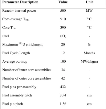
Table 1: DLFR Core Specifications ... 7

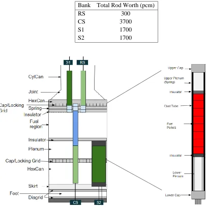
Table 2: Total rod worth in each control bank ... 10

Table 3: Eigenvalue results for nominal case from SERPENT and DIF3D ... 25

Table 4: Reactivity feedback coefficients for DLFR ... 28

Table 5: Breakdown of uncertainty in k∞ for an inner assembly from SERPENT ... 32

vi LIST OF FIGURES

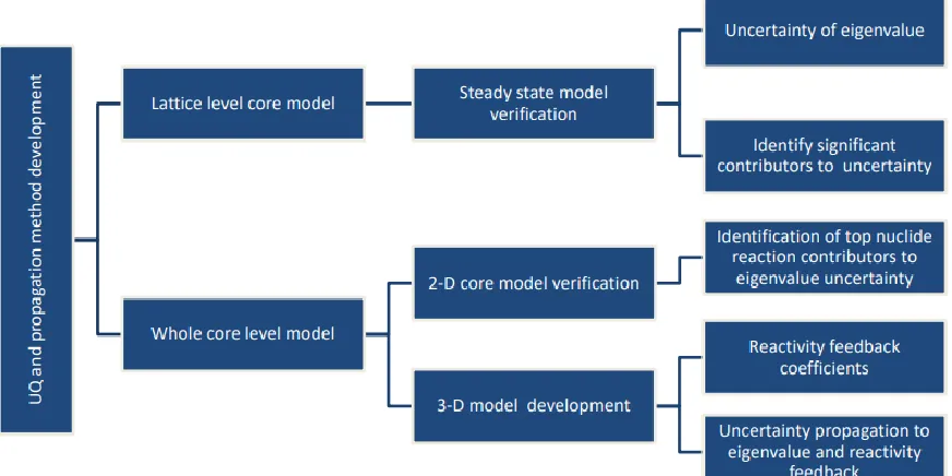
Figure 1: Plan of work overview ... 3

Figure 2: Overview of methodology and computational tools ... 3

Figure 3: Conceptual Vertical (left) and horizontal (right) cross sections of the DLFR primary system showing core and SG layouts [4] ... 6

Figure 4: Radial layout of the DLFR reactor core. S1, S2, CS and RS represent the safety system 1, safety system 2, control system and regulation system employed within the reactor core. The assemblies are identified with coordinates representing ring and assembly numbers. ... 8

Figure 5: DLFR fuel subassembly radial layout [4] ... 9

Figure 6: Simplified axial layout of the fuel assembly (left) and the fuel pin (right) as modelled ... 10

Figure 7: DLFR core (a) and fuel assembly (b) models in SERPENT-2.0 ... 11

Figure 8: Conventional cross-section generation methodology in ARC (UFG and BG refer to Ultra Fine Group and Broad Group, respectively) ... 14

Figure 9: Schematic representation of the improved cross-section generation methodology .... 15

Figure 10: 1D cylinder representation of the fuel assembly ... 17

Figure 11: Sources of uncertainties in a reactor and system design ... 19

Figure 12: 2D Assembly wise power distribution for 1/3rd core ... 26

Figure 13: Flux distribution for central assembly (1, 1) ... 27

Figure 14: Sensitivity of inner core assembly (1, 1) kinf at BOC ... 30

Figure 15: Uncertainty of inner core assembly (1, 1) kinf at BOC ... 30

Figure 16: Sensitivity of inner core assembly (1, 1) kinf at EOC ... 31

Figure 17: Uncertainty of inner core assembly (1, 1) kinf at EOC ... 31

vii Figure 19: Uncertainty contribution from the main 5 isotopes at BOC. Solid lines for

SERPENT results, dashed lines for PERSENT results (solid lines for SERPENT results,

dashed lines for DIF3D results). ... 34

Figure 20: Uncertainty breakdown of Doppler reactivity feedback ... 36

Figure 21: Uncertainty breakdown of radial feedback coefficients ... 37

Figure 22: Uncertainty breakdown on fuel and feedback coefficients ... 37

Figure 23: Uncertainty breakdown of structure feedback coefficient ... 38

Figure 24: UTOP peak temperatures ... 42

1

CHAPTER

INDTRODUCTION

In 1951, development of the world’s first power producing fast breeder reactor - the Experimental Breeder Reactor (EBR-I) - left a historic landmark in the nuclear technology timeline [1]. Since then, fast reactors research has gained tremendous momentum around the world with renewed interest in development of Generation-IV type nuclear reactors. In a collaborative effort led by Generation-IV International Forum (GIF) aimed towards meeting the rapidly growing energy needs of the world, six new advanced reactor designs were selected [2]. These reactors systems included the Very High Temperature Reactor (VHTR), Gas-cooled Fast Reactor (GFR), Sodium-cooled Fast Reactor (SFR), Lead-Sodium-cooled Fast Reactor (LFR), Molten Salt Reactor (MSR), and Supercritical Water-cooled Reactor (SCWR) [2]. Amongst these, LFRs emerged as one of the most promising, proliferation resistant, and sustainable reactor concepts offering safety and economic advantages over other fast reactor technologies [3].

Enhanced safety features of LFRs such as relatively inert coolant, retention of hazardous radionuclides including iodine and cesium in coolant, and high boiling point of lead at 1743 o_C

make it an optimal coolant choice for reactors with Heavy Liquid Metal Coolant (HLMC) [2, 3].

2 Lack of vigorous exothermic reaction between the coolant and air or water, favorable heat transfer, and excellent neutronic properties provide an opportunity for an open fuel lattice without compromising core pressure and neutron efficiency [3]. The compact vessel design from absence of an intermediate cooling circuit further accentuates the economic competitiveness of LFRs.

However, there is a significant lack in plant operational history of HLMC type reactors, compared to conventional Light Water Reactor (LWR) designs. As such, regulatory acceptance of LFRs relies on the quality and accuracy of reactor safety analysis. Safety parameters determined using modern codes have a direct impact from nuclear data and other uncertainties. Evaluation of these uncertainties will lead to a better understanding of their impact on reactor core design and identification of the design safety limits.

3 Figure 1: Plan of work overview

4 In addition to above, an LFR reactor system is developed here to set up framework for propagation of such uncertainties through a system and assess their impact on safety parameters like fuel and clad temperatures.

5

CHAPTER

CORE DESING, SPECIFICATION, AND

MODELLING

2.1Demonstration Lead-cooled Fast Reactor Design

The Demonstration Lead-Cooled Fast Reactor (DLFR) was originally conceptualized by Westinghouse Electric Company (WEC) as an option for the advanced demonstration and test reactor study conducted by the Department of Energy (DOE). WEC developed the DLFR in collaboration with Argonne National Lab (ANL) and the Italian National Agency for New Technologies, Energy and Sustainable Economic Development (ENEA) with the objective of providing an insight into feasibility and basic performance of the LFR technology.

The motivation for selecting this specific reactor design for this research is based on DLFRs capabilities of providing a commercially viable reactor technology. It features a compact, pool-type design rated at 500 MW th, which is suitable for modular construction and enhanced economic benefits. In addition to being one of the first commercial LFR demonstration designs in the past decade in United States, the DLFR design was optimized for feasible inspection, maintenance and replacement of the primary system and components [4].

6 The pool type layout of the primary system with reactor coolant pumps (RCPs) incorporated into the steam generator (SG) is provided in Figure 3. As explained in reference [4], designs of the SGs for DLFR were adopted from the ELSY reactor design. RCPs draw the coolant from hot pot pool near the core to the SGs which are located above the core. Cold lead flows back through the downcomers entering the core from the bottom. The main reactor vessel contains all primary components immersed in liquid lead. All cladding and other in-core components are made of authentic 15-15Ti stainless steel, which is qualified for use in a nuclear reactor with oxide fuel. In addition, the entire main vessel, comprising of the core barrel and outer wall, is made of stainless steel class AISI 316L. Table 1 summarizes relevant design specifications for core modelling complimenting the information provided in this section.

7 Table 1: DLFR Core Specifications

Parameter Description Value Unit

Reactor thermal power 500 MW

Core-average Tout 510 o C

Core T in 390 o C

Fuel UO2 -

Maximum 235U enrichment 20 %

Fuel Cycle Length 12 Months

Average burmup 100 MWd/kgHM

Number of inner core assemblies 34 -

Number of outer core assemblies 42 -

Fuel pins per assembly 432 -

Fuel assembly pitch 30.4 cm

Fuel pin pitch 1.36 cm

2.1.1 Reactor Core

DLFR reactor core operates on a 12 month fuel cycle, using uranium oxide (UO2) as fuel however

8 Figure 4: Radial layout of the DLFR reactor core. S1, S2, CS and RS represent the safety system 1, safety system 2, control system and regulation system employed within the reactor core. The

assemblies are identified with coordinates representing ring and assembly numbers.

9 Figure 5: DLFR fuel subassembly radial layout [4]

2.1.2 Control Systems

DLFR is controlled using a unique set of control rods called finger absorber rods (FARs) separated into four banks – safety system 1 (S1), safety system 2 (S2), regulation system (RS), and control system (CS), also shown in Figure 4. Each bundle of these absorber pins contain up to 90% 10

10 Table 2: Total rod worth in each control bank

Bank Total Rod Worth (pcm)

RS 300

CS 3700

S1 1700

S2 1700

Figure 6: Simplified axial layout of the fuel assembly (left) and the fuel pin (right) as modelled

2.2Core Modelling

11 calculations on homogenized 0D mixture geometry [6]. However, bearing in mind the complexity of the DLFR fuel assembly with presence of FARs in the central beam tube, Monte Carlo code SERPENT-2.0 is considered for lattice calculations instead [7]. The purpose of using Monte Carlo code at this stage is to truly capture the heterogeneity effects of DLFR fuel assembly and quantify the difference between the explicit model in SERPENT and homogeneous model in MCC-3.1. The reference results were obtained from transport code ERANOS using ECCO [8]. This section provides further information on these codes, and any modelling variations for properly adapting the available tools.

The DLFR models in SERPENT-2.0, shown in Figure 7, uses cross-sections generated from nuclear data library ENDF/B-VII.0.

Figure 7: DLFR core (a) and fuel assembly (b) models in SERPENT-2.0

The 3D core DLFR model, (Figures 4) is developed in ARC suite. Within ARC, cross-sections are generated using MCC-3.1 coupled with 2D Sn transport solver code TWODANT [6, 9]. These

12 safety rods (S2) withdrawn below core (Figure 6). An axial temperature gradient, provided by ENEA, is maintained for all core components above, below and at core level during the reactor core model setup [4]. Consequently, temperature dilatation effects on all structural geometry and densities was considered for correct neutronic simulation at operating temperatures. All dimensions and densities were carefully adjusted by factors governed by their respective coefficient of linear thermal expansion described by 𝛼𝑇 =

1 𝐿(

𝑑𝐿

13

CHAPTER

CROSS-SECTION GENERATION METHODS

In core calculations, the first step is to generate multi-group cross-sections. This calculation is performed using lattice codes which solves the multi-group Boltzmann transport equation given as 1 𝜈 𝛿𝜙 𝛿𝑡 + Ω̂ ∙ ∇𝜙 + Σ𝑡(𝑟, 𝐸)𝜙(𝑟, 𝐸, Ω̂, 𝑡) = ∫ 𝑑Ω̂′_{∫ 𝑑𝐸}′_Σ 𝑆(𝐸′→ 𝐸, Ω̂′ → Ω̂)𝜙(𝑟, 𝐸′, Ω̂, 𝑡) ∞ 0 4𝜋 + 𝑠(𝑟, 𝐸, Ω̂, 𝑡) (1) where, (a) 1 𝜈 𝛿𝜙

𝛿𝑡 = Rate of change in neutron population

(b) Ω̂ ∙ ∇𝑛 = Leakage

(c) Σ_𝑡(𝑟, 𝐸)𝑛(𝑟, 𝐸, Ω̂, 𝑡) =Loss due to collision

(d) ∫ 𝑑Ω̂′∫ 𝑑𝐸′Σ𝑆(𝐸′→ 𝐸, Ω̂′ → Ω̂)𝑛(𝑟, 𝐸′, Ω̂, 𝑡) ∞

0

4𝜋 = Gain due to in scattering

(e) 𝑠(𝑟, 𝐸, Ω̂, 𝑡) =Rate of source of neutrons

14 Using flux solutions from the transport equation, condensed multi-group, and self-shielded cross-sections are obtained using nuclear data files. It is important to preserve reaction rates when these condensing cross-sections. In MCC-3.1, P1 multi-group transport equation is solved for generation

the multi-group neutron cross-sections using either homogeneous, 1D heterogeneous slab or cylinder geometry. The cross-sections in ultrafine group (~2000) are self-shielded by numerical integration of point wise cross-sections based on narrow resonance approximation [6].

Conventional method for cross-section generation in ARC using the multi-group cross-section generation code MCC-3.1 for obtaining self-shielded cross-sections is shown in Figure 8. First, the core is represented with a 0D mixture geometry for each assembly. MCC-3.1 calculates condensed region wise self-shielded 230 ultrafine group (UFG) cross-sections using 2082 groups master isotopic library and provides them to TWODANT [6]. TWODANT performs transport calculations on an equivalent R-Z model of the core to obtain region-wise flux solutions with 230 UFG cross-sections [9]. Finally, MCC-3.1 generates region-wise 33 broad group (BG) condensed cross-sections using the UFG flux solutions obtained in the previous step [6].

Figure 8: Conventional cross-section generation methodology in ARC (UFG and BG refer to Ultra Fine Group and Broad Group, respectively)

However, one of the main challenges of modelling DLFR using ARC is during cross-section generation process due to subassembly geometry. The DLFR subassemblies have radial

Step 1: MCC-3.1

Generates condensed 230UFG cross-sections from 2082 groups master library with mixture composition

Step 2: TWODANT

Fine group flux calculations in RZ

Step 3: MCC-3.1

15 heterogeneity within the subassembly due to presence of absorber material in the central beam tube (figure 5). The conventional cross-section generation method in MCC-3.1 uses complicates the process of generating properly self-shielded cross-sections considering the 0D homogenized geometry utilized in step 1 (Figure 8). Intermediate steps were necessary to obtain properly self-shielded cross-sections reflecting the true material distribution the fuel assembly. This involved improved implementation of the conventional cross-section generation methodology. The primary purpose of this method is the proper treatment of the self-shielding effects due to absorber material in the center of fuel assemblies. Figure 9 provides a schematic understanding of the improved cross-section generation methodology.

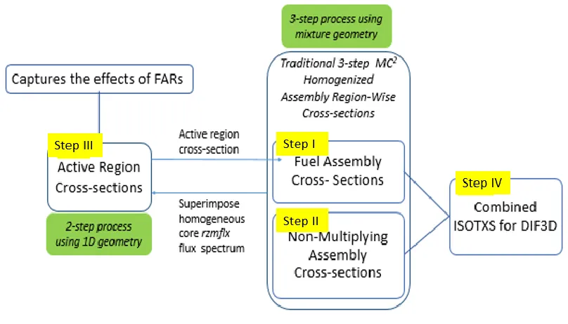
16 I. Fuel assembly cross-sections

i. A DLFR fuel subassembly (Figure 6) is represented with 0D homogenized axial regions in mixture geometry.

ii. Similar to step 2 in Figure 8, the fuel subassembly is represented with an equivalent RZ model in TWODANT to generate region-wise flux solutions in axial direction. iii. Condensed 33 BG axial leakage corrected cross-sections are generated by MCC-3.1

using flux spectrum from step ii for one fuel subassembly type. Steps i-iii are then repeated for each fuel subassembly type. In DFLR, there are six different fuel subassembly types between inner and outer core, i.e. inner core assembly without FAR, inner core assemblies with RS, S1, and CS type FARs, outer core assembly without FAR, outer core assemblies with S1 type FARs. Total of six separate cross-section calculations are performed at this stage.

II. Non-multiplying assembly cross sections

i. Cross-sections for non-multiplying assemblies (shield, reflectors and S2 safety system) are generated using the traditional process outlined in Figure 8. The core is represented using homogenized mixture geometry for different subassemblies. The region-wise flux solutions from TWODANT are saved in an rzmflx file.

III. Fuel assembly active region cross sections

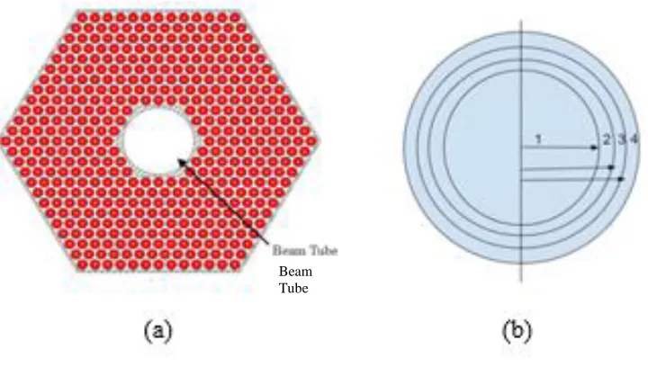
17 transport solutions of step v. This approach simultaneously allows taking into account the heterogeneity effects in the fuel region and leakage effect between regions in core. Figure 10b shows the 1D fuel assembly model where the beam tube and fuel rings in Figure 10a, correspond with equivalent cylindrical rings 1, 2, etc. Each cylinder is subdivided into 1D sub-cylinders separating the materials contained within the original cylinder. More details on this methodology can be found in reference [13].

Figure 10: 1D cylinder representation of the fuel assembly

IV. Merged cross-sections

i. Different region cross-sections from all subassemblies are merged into one ISOTXS format file for all other computations.

18

CHAPTER

UNCERTAINTY QUANTIFICATION AND

PROPAGATION

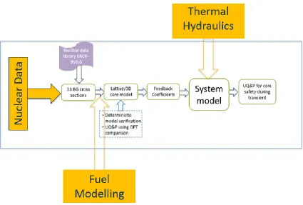
Quantifying the uncertainties in a new system design is crucial to understanding its safety

capabilities during design based events and accidents. Throughout the core design process, many sources of uncertainties such as those from fuel modelling, thermal hydraulics, etc. can be introduced at different stages of modelling, as seen in Figure 11. Proper handling and

propagation of uncertainties is therefore necessary to establish confidence bounds on core safety and performance parameters. Currently, only nuclear data uncertainties are being considered through the system. This section provides an overview of the uncertainty quantification methodology and the systematic approach followed for propagation of these uncertainties through the reactor system.

19 Figure 11: Sources of uncertainties in a reactor and system design

4.1Sensitivity and Uncertainty Analysis for Steady State

To compute the influence of uncertainties on the output for a given model UQ&P of input uncertainties is needed. In a large or complex model, with multiple perturbed system equations for each input variation, the propagation of uncertainty via sampling-based methods is not feasible. One of the alternatives is a perturbation method which is based on truncating the Taylor expansion of a response parameter [16]. Consider a set of random variables 𝑄 = [𝑄1, 𝑄2, … , 𝑄𝑝]. The first order linear expansion for the model response 𝑓(𝑄) is

𝑓(𝑄) = 𝑦̅ + ∑ 𝑠_𝑖𝛿𝑄_𝑖

𝑝

𝑖=1

(2)

where 𝑦̅ = 𝑓(𝑞̅) and 𝑠_𝑖 = 𝜕𝑓

20 Covariance of 𝑄_𝑖 with 𝑄_𝑗 is expressed as

𝑐𝑜𝑣(𝑄_𝑖, 𝑄_𝑗) = ∫ (𝑞_𝑖−

ℝ

𝑞̅ )(𝑞_{𝑖 𝑗}− 𝑞̅ )𝜌_{𝑗 𝑄}(𝑞)𝑑𝑞 (3)

Where 𝜌𝑄(𝑞) is the probability density function of Q

and the expectation of Q can be defined as 𝔼(𝑄) = 𝑞̅_𝑖.

𝔼[𝑓(𝑄)] = 𝑦̅ ∫ 𝜌_𝑄(𝑞)𝑑𝑞 + ∑ 𝑠_𝑖∫ (𝑞_𝑖− 𝑞̅ )𝜌_{𝑖 𝑄}(𝑞)𝑑𝑞 = 𝑦̅ ℝ𝑝 𝑝 𝑖=1 ℝ𝑃 (4)

Evaluating the integrals in the above equation where the first integral is unity and second is zero, variance of 𝑓(𝑄) is

𝑣𝑎𝑟[𝑓(𝑄)] = 𝔼[(𝑓(𝑄) − 𝑦̅)2_{] (5)}

Using Eq (2),

𝑣𝑎𝑟[𝑓(𝑄)] = ∫(∑ 𝑠𝑖𝛿𝑄𝑖

𝑝

𝑖=1

)2𝜌𝑄(𝑞)𝑑𝑞 = ∑ 𝑠𝑖2𝑣𝑎𝑟(𝑄𝑖) + ∑ ∑ 𝑠𝑖𝑠𝑗𝑐𝑜𝑣(𝑄𝑖, 𝑄𝑗) 𝑝 𝑗=1 𝑗≠𝑖 𝑝 𝑖=1 𝑝 𝑖=1 (6)

This can be rewritten in matrix form, also known as the “sandwich rule”, as

𝑣𝑎𝑟[𝑓(𝑄)] = 𝑆𝑇𝐷𝑆 (7)

where D is a covariance matrix for Q and S the sensitivity matrix. Determining the sensitivity coefficients of the response parameter using computational tools is the key factor to this approach [16].

21 theory (GPT) based method was used for building a deterministic model. GPT uses deterministic sensitivity and uncertainty methods to compute sensitivity coefficient Sρ to relate relative change of an integral core parameter (such as multiplication factor) to the relative change in multi-group nuclear data, σg. Once the sensitivity matrix (𝑆_𝑖) associated with each integral parameter is obtained, the total contribution of uncertainties attributed to these coefficients can be determined using correlations and covariance matrices.

For a given core parameter Δρi, the sensitivity coefficient 𝑆_𝜌 is defined as:

𝑆𝑅 = [ 𝑆₁ ⋮ 𝑆𝑖 ⋮ 𝑆𝑁]

𝑓𝑜𝑟 1 ≤ 𝑖 ≤ 𝑁 (8)

where 𝑁 = Nuclide-reaction number × energy groups. For example, for 235U fission reaction for 33 energy groups, 𝑁 = 1 × 33. Each sensitivity coefficient is

𝑆𝑗,𝑥,𝑔= 𝜕𝜌 𝜌⁄ 𝜕𝜎_{𝑗,𝑥,𝑔}⁄𝜎_{𝑗,𝑥,𝑔} = 𝜕𝜌 𝜕𝜎_{𝑗,𝑥,𝑔} 𝜎𝑗,𝑥,𝑔

𝜌 (9)

where j, x and g represent the isotope, the cross-section type, and the energy group, respectively.

22

𝐷 = (𝐷_𝑥,𝑗) =

[

𝐷11 𝐷12 ⋯ ⋯ 𝐷1𝑁

𝐷₂₁ …

⋮ 𝐷_𝑗𝑗

⋮ ⋯

𝐷_𝑁1 𝐷_𝑁𝑁]

𝑓𝑜𝑟 𝑁 = 33 𝑒𝑛𝑒𝑟𝑔𝑦 𝑔𝑟𝑜𝑢𝑝s_𝑥,𝑗 (10)

Uncertainty 𝐼_𝑖21 for reactivity coefficient 𝜌_𝑖 can be obtained using the “sandwich rule” discussed above:

𝐼_𝑖2 = 𝑆_𝑖𝑇𝐷𝑆_𝑖 (11)

Using the above describe GPT methodology, impact of nuclear data uncertainty is studied on lattice level as well as used to quantify uncertainty in reactivity feedback coefficients. The focus of this study is placed on five different feedback coefficients including Doppler coefficient, radial expansion coefficient and fuel/coolant/structure density worth. The feedback coefficient 𝛼 is obtained as a change in reactivity between base and perturbed core states caused by a change in core parameters (temperature/density/pitch). The sensitivity 𝑆_𝛼,𝜎of a given feedback coefficient 𝛼 to perturbations in nuclear data can be calculated from sensitivity of reactivity change 𝜌 by 𝑆_𝜌,𝜎𝑗 = 𝜕𝜌𝑗

𝜕𝜎𝑖,𝑥,𝑔

𝜕𝜎𝑖,𝑥,𝑔

𝜌𝑗 for base (j=1) and perturbed (j=2) cases. The indices i, x and g represent the

isotope, the cross-section type and the energy group respectively. For Doppler coefficient, base case obtains the sensitivity of reactivity (𝑆_𝜌,𝜎1 _{) to nuclear data perturbations at nominal} temperature. Similarly, perturbed case provides sensitivities (𝑆_𝜌,𝜎2 ) at Doppler temperature. Then, Eq. 1 is used to obtain sensitivity of feedback coefficient 𝑆𝛼,𝜎 by combining 𝑆𝜌,𝜎1 and 𝑆𝜌,𝜎2 using the reactivity change (Δ𝜌 = 1

𝑘1−

1

𝑘2) from the base to the perturbed case [21]:

1 _{It should be noted that, mathematically 𝐼}

23

𝑆𝛼,𝜎 =

𝑆_𝜌2_2,𝜎

𝑘2 −

𝑆_𝜌1_1,𝜎 𝑘1 Δ𝜌

(12)

The total uncertainty 𝐼𝑛2of 𝛼 can now be described using equation 11.

Sensitivity matrix of the eigenvalue and reactivity feedback coefficients is obtained using ANL perturbation theory based code PERSENT. PERSENT employs the adjoint-based sensitivity analysis to generate the sensitivity coefficients. In this methodology, the sensitivity functions are evaluated using adjoint variables without solving perturbed system equations for each input parameter change. PERSENT uses variational methods for the adjoint-based sensitivity analysis where the solution of the corresponding adjoint transport equation is used to compute changes in eigenvalue based on perturbations in the cross section. [18, 19].

The GPT methodology applied on ARC results to compute total contribution on uncertainties is verified using the GPT capabilities implemented within SERPENT. The sensitivity coefficients in SERPENT are generated using a collision-history based approach explained further in reference [20].

4.2 Variance-Covariance Data

24

CHAPTER

RESULTS AND DISCUSSION

The preliminary nature of this work makes it necessary to quantify the extent to which the results can be trusted. In absence of experimental data, verification methods such as code-to-code comparison eliminate errors and ensure that the model behaves as the user intended. Therefore, lattice models developed lattice models developed here using deterministic ARC codes are verified against Monte Carlo code SERPENT for various core performance parameters including criticality, power, and flux profiles.

This section first presents the lattice level criticality results from base case models developed in MCC-3.1 which are verified with an explicit model in SERPENT. This quantifies the difference between the SERPENT and ARC in terms of reactivity. Upon establishing an acceptable level of difference at assembly level, a nominal case is developed for whole core model verification as explained in the following sections.

5.1 Lattice Model Verification

Initial results obtained from SERPENT and MCC-3.1 using models described in Chapter 2 are summarized in Table 3, where BOC/EOC refer to Beginning of Life, Beginning of Cycle, End of

25 Cycle, and End of Life in core composition, respectively. Neutron population in SERPENT is set to 100000 with 500 active and 50 inactive cycles. The models are at all rods out core condition.

Table3: Eigenvalue results for nominal case from SERPENT and DIF3D

SERPENT MC2-3.1 Δpcm % δk/k

Outer Core k∞

BOC 1.28194±0.00014 1.28121 44.4 -0.05

EOC 1.25681±0.00015 1.25813 -83.5 0.10

SERPENT DIF3D

2D Core k∞

BOC 1.17683±0.00018 1.1688 583.8 0.66

EOC 1.15126±0.00017 1.1437 574.2 0.91

Eigenvalues at assembly level show less than 100 pcm difference between the fully heterogeneous in SERPENT model and the homogenized assembly model in MCC-3.1. However, this difference at 583.8 pcm is significantly larger on 2D core level. Comparing the two models, the source of the observed differences is attributed to the two different methods of cross-section generation between SEPRENT and MCC-3.1 along with the explicit model used in SERPENT.

26 Figure 12: 2D Assembly wise power distribution for 1/3rd core

Additionally, Figure 13 provides comparison of the flux distribution in the central fuel assembly from SERPENT and DIF3D. Although a good overlap is seen between the two results, the difference in peak values is noticeable based on how the energy bins are tallied. The Monte Carlo relative statistical error from SERPENT for all flux data is to order of 10-3

.In DIF3D, ANL 33

27 Figure 13: Flux distribution for central assembly (1, 1)

5.2 Whole Core Level

A full core steady state model is developed in DIF3D for the purpose of this work. However, as explained in Chapter 3, an improved method for cross-section generation was implemented considering the axial and radial heterogeneity of the DLFR core. To demonstrate the improvements from cross-section generation methodology and understand reactivity feedback responses to variations in core temperature (Chapter 4), 3-D full core is modelled in DIF3D.

28 differences, the improved cross-section generation approach is adapted for assessing all core performance parameters. Using the new cross-section generation method, a keff of 1.03321 is

obtained at BOC. Future work is underway to verify the improved cross-section generation methodology as explained in Chapter 5.

This model is then used to generate selected five reactivity feedback coefficients which are summarized in Table 4 below.

Table 4: Reactivity feedback coefficients for DLFR

Feedback

Parameter

Perturbation Type

Degree of Variation Reactivity [pcm] Coefficient (pcm/K) Doppler Fuel temperature (Nominal at 926 o_C)

+500 oC -713.51 -0.9240

Radial Expansion

Core pitch +2.5% -851.31 -0.8314

Structure Density

15-15Ti SS Density in active region

-5% 116.53 0.1551

Coolant Density

Lead Density in active region

-5% -70.51 -0.1720

Fuel Density Fuel Density -5% -1423.98 -2.1450

self-29 shielding effects a depression in flux in vicinity of resonance peaks will also contribute to the negative reactivity. In radial expansion coefficient, core pitch is expanded while preserving mass of fuel and structure. Increase in coolant volume inside the core with increased moderation of neutrons leads to addition of net negative reactivity. Similarly, when fuel density expands, the fissile nuclide concentration is also reduced adding negative reactivity to the core. For coolant density expansion reactivity feedback, net negative reactivity is added based on the competing effects of positive reactivity from reduced amount of coolant per unit volume, negative reactivity from increased leakage, and positive reactivity from decreased neutron capture. The coolant reactivity feedback is design dependent. For structure density expansion coefficient, large positive reactivity is added. Positive reactivity is expected since decrease in clad density leads to decreased interaction between neutrons and steel.

5.3 Uncertainty Quantification

5.3.1 Lattice Level

30 Figure 14: Sensitivity of inner core assembly (1, 1) kinf at BOC

31 Figure 16: Sensitivity of inner core assembly (1, 1) kinf at EOC

32 Table 5: Breakdown of uncertainty in k∞ for an inner assembly from SERPENT

Rank Uncertainty Contribution (%)

Nuclide/nuclide reaction BOC Nuclide/nuclide reaction EOC

1 235U(n,γ)/ 235U(n,γ) 65.8 235U(n,γ)/ 235U(n,γ) 60.9

2 238U(n,n’)/ 238U(n,n’) 19.1 238U(n,n’)/ 238U(n,n’) 23.8

3 238U(n,γ)/ 238U(n,γ) 5.11 238U(n,γ)/ 238U(n,γ) 6.3

4 235U fission/ 235U fission 1.74 235U fission/ 235U fission 1.72

5 16O (n,n)/16O (n,n) 0.09 56Fe (n,n)/56Fe (n,n) 1.52

Total contribution to k∞ 1.50 1.35

Based on the sensitivity results, uncertainties for nuclide reaction pairs were computed using the “sandwich rule” described in Chapter 4. The largest contribution to uncertainty in kinfcomes from

heavy metals - 235_{U and} 238_{U. Both quantities have a decreasing trend as the core depletes however}

it is important to note that the uncertainty trend remains consistent. Positive sensitivity profiles implies a positive linear relationship between perturbations in the input and its effect on the output, whereas negative profiles show a non-linear relationship between the output and the input. For the negative profiles, as the input is increased, the output shows a decrease and vice versa.

33 determine the contribution of uncertainty to the kinf. The correlations show the statistical

relationship between two nuclide reaction types. 235U capture-235U capture reaction pair has a strong positive correlation – as is also the case for 238U -inelastic scattering pair. The multiplication factor is noticeably sensitive to perturbation in the 235_{U fission and} 235_{U capture cross sections}

which lead to a large uncertainty contribution to the multiplication factor based on their positive correlation coefficients.

5.3.2 Uncertainty Quantification on 2D Core

34 Figure 18: Sensitivity profile for top 5 cross-sections to which keff is most sensitive at BOC

(solid lines for SERPENT results, dashed lines for DIF3D results).

Figure 19: Uncertainty contribution from the main 5 isotopes at BOC. Solid lines for SERPENT results, dashed lines for PERSENT results (solid lines for SERPENT results, dashed lines for

35 A substantial amount of uncertainty contribution from 235U capture-235U capture reaction pair is evident in Figure 19. This is not a surprising result considering the high enrichment in the core at BOC. The 238U inelastic-238U inelastic reaction pair provides the next largest contribution. Contribution from the top two nuclide reaction pairs accounts for 85% of the uncertainty in keff

when the respective cross-section was perturbed by 1.01. In addition, there is good comparison between the uncertainty profiles from SERPENT and PERSENT based on the trends observed in Figure 19, although the values are not distinguishable in the lower energy range. This is likely due to the low flux in that region as shown in Figure 13.

5.3.3 UQ&P in Reactivity Feedback

Total uncertainty of each feedback coefficient from perturbations in nuclear data is given in Table 6. Largest uncertainties are observed for the fuel density expansion followed by coolant expansion and Doppler.

Table 6: Total uncertainty of steady state feedback coefficients

Breakdown of the total uncertainty of neutronic feedback coefficients from Table 6 is provided in Figures 20-23 to show contribution from various reaction channels. A large contribution is observed for fuel density and Doppler reactivity feedback coefficient at BOC composition where majority of the uncertainty is seen to originate from U-238 inelastic scattering in high-energy range above 1 MeV. This can be associated with the significant sensitivity of the feedback coefficients

Δρ Doppler Δρ Fuel Δρ Coolant Δρ Structure Δρ Radial Expansion

36 to the perturbations in U-238 inelastic reaction cross-section and strong reaction channel correlation in this energy range. For core radial expansion and structure feedback (Figs. 6b and 7b, respectively), U-235 fission and capture cross-section become significant in epithermal range. Decreased structural density leads to reduced moderation, increased fission, and addition of uncertainty contribution from U-235. Similarly, expansion of core pitch will increase coolant volume inside the reactor and add negative reactivity.

37 Figure 21: Uncertainty breakdown of radial feedback coefficients

39

CHAPTER

CONCLUSION AND FUTURE WORK

6.1 Concluding Remarks

Uncertainty quantification and sensitivity analysis are key parameters in reactor design. In this work, a method is developed for quantification of nuclear data uncertainties through lead-cooled fast reactors using best estimate methods. The uncertainty and sensitivity profiles are generated using the Monte Carlo code SERPENT with GPT and the ANL code package for fast reactors, ARC, for the equilibrium core composition. Impact of these uncertainties is assessed on core performance and safety parameters including reactivity feedback. It is observed that multiplication factor is most sensitivity to perturbations in 235U-fission cross-section, 235U-ν and 238U-capture cross section. This is followed by 239Pu and 238U-capture cross sections as the fuel experiences burnup. Additionally, at BOC composition, 238U-elastic, 238U-inelastic and 238U-capture cross-sections are identified as top contributors to the total uncertainty in reactivity feedback coefficients.

Furthermore, this work provides a framework for propagation of nuclear data uncertainties through LFR system model described in the next chapter.

40 6.2Future Work

In order to propagate nuclear data input uncertainties through transients, uncertainties in feedback coefficients are established. Feedback coefficients can then be perturbed with those standard deviations to evaluate core safety capabilities.

6.2.1 Reactor System Model

In its initial stages, the DLFR system model is envisioned to include a primary heat transfer system and emergency heat removal system (DRACS) driven by natural circulation. The model is generated in the limited, non-commercial version of SAS4A/SASSYS-1, called MiniSAS developed by ANL [14]. MiniSAS is compiled from the same source code as SAS4A/SASSYS-1 while excluding some capabilities such as severe accident modelling [14]. The overall system design is adapted from the sodium fast reactor ABR1000 system for preliminary safety analysis of DLFR [15]. In the current model, coolant flows from hot pool to heat exchangers and is dumped back into cold pool. Primary pumps then feed cold lead through the core extracting heat from the reactor. A once through steam generator is also modelled in the secondary system. In order to make the ABR 1000 model more suitable for LFR system, some design parameters were updated from existing LFR data including core flow rate of 28560 kg/s, coolant inlet temperature at 663.3 K and core power of 500 MWth in nominal state [4]. A more comprehensive list of system specification

and coolant flow schematic is provided in Appendix B.

41 pin is discretized into 10 radial temperature nodes and 20 axial segments. A simple radial expansion model from MiniSAS is incorporated to account for core bowing effect.

6.2.2 Transient Simulation

After establishing steady state, reactivity feedback and temperature increase during the unprotected transient over power (UTOP) accident is evaluated using MiniSAS. The transient is simulated with reactivity insertion of $0.5 over 15 second to represent inadvertent rod withdrawal accident with reactivity ramp. No safety or control rods are envisioned to enter the core during this event. The pumps are expected to operate at full speed with heat transfer occurring via primary loop and DRACS. Remaining parameters were anticipated to be those at nominal state. Peak fuel, clad and coolant temperatures are selected as the quantities to interest to provide an insight into core safety during accidents as shown in Figure 24.

The reactivity ramp during transient increases fuel temperature (Figure 24) but a large negative Doppler is immediately triggered to counter the positive reactivity excursion (Figure 25). Additional negative reactivity feedback from core flowering effect compensates for the remaining positive reactivity inserted during transient. Another main concern during UTOP transient is the fuel peak temperature, which however remains well below the melting point of 3200K for UO2

42 Figure 24: UTOP peak temperatures

44 REFERENCES

1. Alemberti et. al, “Overview of lead-cooled fast reactor activities,” Progress in Nuclear Energy, 77, pp. 300-307 (2013).

2. G.Grosch, “Generation IV Systems,” GIF Portal - Home, (2013)

3. Nuclear Energy Agency. “Handbook on Lead-bismuth Eutectic Alloy and Lead

Properties, Materials Compatibility, Thermal-hydraulics and Technologies”. Technical report NEA No. 7268, OECD, 2015

4. “Demonstration Lead-cooled Fast Reactor,” Contract DE-AC02-06CH11357, RT-TR-15-30, Westinghouse Electric Company LLC, March 8, (2016).

5. B. J. Toppel et. al., “The Argonne Reactor Computation (ARC) System,” Technical report, ANL-7332, Argonne National Lab, (1967).

6. M.C. Smith et al. “MC2 -3: Multigroup Cross Section Generation code for Fast Reactor Analysis,” Technical Report ANL/NE-11-41, (2013).

7. J. Leppanen et al. “The SERPENT Monte Carlo code: Status, development and applications in 2013”. Annals of Nuclear Energy, vol. 82, 2015, pp. 142-150. 8. J.M. Ruggieri, et. al., “ERANOS 2.1 : International Code System for GEN IV Fast

Reactor Analysis,” Proceeding of ICAPP, Nevada USA, (2006).

9. R. Alcouffe et al., “User’s Guide for TWODANT: A Code Package for

Two-Dimensional, Diffusion-Accelerated Neutral-Partical Transport,” LA-10049-M, LANL, (1984).

10. K.L. Derstine, “Dif3D: A Code To Solve One-, Two- and Three- Dimensional Finite-Difference Diffusion Theory Problems,” Technical report ANL-82-64, ANL, (April 1984).

45 12. Del Nevo et al., “Modelling and Analysis of Nuclear Fuel Pin Behavior for Innovative

Lead Cooled FBR,” Technical Report ADPFISS-LP2-054, (2014).

13. Lee et al., “Improved Reactivity Worth Estimation of MC2-3/DIF3D in Fast Reactor Analysis,” Proceedings of ANS Sumer Meeting, San Antonio, Texas, (2015).

14. T. H. Fanning et al., “SAS4A/SASSYS-1 Code Improvements for FY 2016,” ANL-ART-75, (2016).

15. N. Stauff et al., “Uncertainty Quantification of ABR Transient Safety Analysis,” Proceedings of ANS Best Estimate Plus Uncertainty (BEPU) International Conference, Lucca, Italy, (2018).

16. R.C. Smith. Uncertainty Quantification. Siam, Philadelphia, 2014.

17. M. Herman et al. “AFCI-2.0 Neutron Cross Section Covariance Library”. Technical report BNL-94830-2011, BNL, March 2011. doi:10.2172/1013530.

18. M.A. Smith et al. “VARI3D & PERSENT: Perturbation and Sensitivity Analysis”. Technical report ANL/NE-13/8, ANL, June 2013.

19. K.F. Laurin-Kovitz and E.E. Lewis. “Variational Nodal Transport Perturbation Theory”. Nuclear Science and Engineering, vol. 123, no. 3, 1996, pp. 369-380.

20. M. Aufiero et al. “A collision history-based approach to sensitivity/perturbation

calculations in the continuous energy Monte Carlo code SERPENT”. Annals of Nuclear Energy, vol. 85, 2015, pp. 245-258.

21. B. M. Adams et al., “Dakota, A multilevel Parallel Object-Oriented Framework for Design Optimization, Parameter Estimation, Uncertainty Quantification, and Sensitivity Analysis: version 6.9 Manual,” (2018).

46 23. G. Grasso et al., “The Core Design of ALFRED, A Demonstrator for the European Lead

cooled Reactors,” Nuclear Engineering and Design, 278, pp. 287-301 (2014). 24. F. Bostelmann et al. “Benchmark for Uncertainty Analysis in Modelling (UAM) for

48 Appendix A

System model specifications for the currently DLFR system in Mini SAS System Components Description

Coolant Flow rate 28560 kg/s

Coolant inlet 663K

Fuel/Coolant Type Oxide/Lead

Core Channels 2 channels: IC and OC

Heat Exchanger (HX) 4 identical HX – 1 is modelled in SAS

Steam Generator Once through SG

Pump

Normalized pump head vs. time provided for the intermediate and primary pumps Direct Reactor Auxiliary

Cooling System (DRACS)

Emergency cooling system

Beta values

49 Appendix B

33 energy group stricture adapted with MCC-3.1, SERPENT-2.0 and COMMARA-2.0 with energies in eV

Group MCC-3.1 (ANL) SERPENT-2.0 COMMARA-2.0

1 1 1.4191E+07 1.964033E+07 1.964033E+07

2 2 1.0000E+07 1.000000E+07 1.000000E+07

3 3 6.0653E+06 6.065307E+06 6.065307E+06

4 4 3.6788E+06 3.678794E+06 3.678794E+06

5 5 2.2313E+06 2.231302E+06 2.231302E+06

6 6 1.3534E+06 1.353353E+06 1.353353E+06

7 7 8.2085E+05 8.208500E+05 8.208500E+05

8 8 4.9787E+05 4.978707E+05 4.978707E+05

9 9 3.0197E+05 3.019738E+05 3.019738E+05

10 10 1.8316E+05 1.831564E+05 1.831564E+05

11 11 1.1109E+05 1.110900E+05 1.110900E+05

12 12 6.7379E+04 6.737947E+04 6.737947E+04

13 13 4.0868E+04 4.086771E+04 4.086771E+04

14 14 2.4787E+04 2.478752E+04 2.478752E+04

15 15 1.5034E+04 1.503439E+04 1.503439E+04

16 16 9.1188E+03 9.118820E+03 9.118820E+03

17 17 5.5308E+03 5.530844E+03 5.530844E+03

18 18 3.3546E+03 3.354626E+03 3.354626E+03

19 19 2.0347E+03 2.034684E+03 2.034684E+03

20 20 1.2341E+03 1.234098E+03 1.234098E+03

21 21 7.4852E+02 7.485183E+02 7.485183E+02

22 22 4.5400E+02 4.539993E+02 4.539993E+02

23 23 2.7536E+02 3.043248E+02 3.043248E+02

24 24 1.6702E+02 1.486254E+02 1.486254E+02

25 25 1.0130E+02 9.166088E+01 9.166088E+01

26 26 6.1442E+01 6.790405E+01 6.790405E+01

27 27 3.7267E+01 4.016900E+01 4.016900E+01

28 28 2.2603E+01 2.260329E+01 2.260329E+01

29 29 1.3710E+01 1.370959E+01 1.370959E+01

30 30 8.3153E+00 8.315287E+00 8.315287E+00

31 31 3.9279E+00 4.000000E+00 4.000000E+00

32 32 5.3158E-01 5.400000E-01 5.400000E-01

50 Appendix C

Sensitivity and uncertainty analysis for DLFR fuel assembly and 2D core model results are presented in this section. BOL/BOC/EOC/EOC refer for beginning of life, beginning of cycle, end of cycle, and end of life, respectively.