Efficient Uncertainty Quantification for a Fast-Spectrum Generation IV Reactor System

Abstract

ELKINS, JASON ROBERT. Efficient Uncertainty Quantification for a Fast-Spectrum Generation IV Reactor System. (Under the direction of Hany S. Abdel-Khalik.)

This research is part of on-going research on the management of uncertainties in simulator predictions for Generation IV systems via optimum experimental design. The focus is on uncertainties originating due to input data. The objective is to devise an algorithmic framework for quantification of uncertainties, identification of their key sources, and ultimately guiding the design of validating experiments for their reduction. An integral part of this research is the development of uncertainty quantification

algorithms for models involving many input data and output responses. This represents the focus of the research reported here.

reactivity and other reactor performance attributes. Currently, we focus on uncertainties originating from cross-section data uncertainties, believed to be of primary significance for fast reactor calculations.

This thesis presents a recent development of an UQ algorithm for increasing the efficiency of UQ to a level that enables its execution on a routine basis with best estimate calculations for various reactor performance attributes. Our objective is to devise an algorithm that can characterize uncertainties in the multitudes of reactor performance attributes as evaluated by reactor simulation tools on a routine basis with reference calculations.

Efficient Uncertainty Quantification for a

Fast-Spectrum Generation IV

Reactor System

by Jason R. Elkins

A thesis submitted to the Graduate Faculty of North Carolina State University

in partial fulfillment of the requirements for the Degree of

Master of Science

Nuclear Engineering

Raleigh, North Carolina 2008

APPROVED BY:

_________________________ ________________________ Dr. Paul J. Turinsky Dr. Agnes Szanto Co-Chair Committee Member

ii

Dedication

Biography

Jason Robert Elkins was born in Greensboro, North Carolina at Moses Cone Hospital on April 26, 1984 to John and Judy Elkins. He received his elementary and secondary education from Liberty Elementary and Middle School located in Liberty, North Carolina. He later attended Eastern Randolph High School of Ramseur, North Carolina and graduated 4th out of 207 students in 2002.

After his high school education, Jason was accepted into the College of Engineering at North Carolina State University of Raleigh, North Carolina. After enrolling into the Department of Nuclear Engineering, his summers consisted of internships at Knolls Atomic Power Laboratory of Schenectady, New York and Duke Energy of Charlotte, North Carolina. He received his Bachelor’s of Science in May 2006 from the Department of Nuclear Engineering, graduating Summa Cum Laude. Following graduation, Jason began work toward a Master’s of Science in Nuclear Engineering under the direction of Dr. Hany S. Abdel-Khalik.

iv

Acknowledgments

Throughout my academic career, I have had an immense amount of support from so many people so please forgive me if I leave someone out. First I want to recognize and thank my parents, John and Judy Elkins, for always providing me with more than enough support to reach all of my goals. During my hardest times at school, I could always count on visiting them for comfort. I would also like to thank my brother, Bret Elkins, for being the most wonderful brother and friend that I could ask for. Finally, I want to thank the soon-to-be Mrs. Elkins, Alex Lucas, for always being there no matter what. It was because of you that I was able to make it through the worst of times and you who created the best.

Table of Contents

List of Figures ... vii

List of Tables ... viii

Nomenclature... ix

1 Introduction... 1

1.1 Purpose... 1

1.2 Core Simulator Background ... 2

1.3 Uncertainty Quantification... 2

1.4 Uncertainty Quantification Techniques ... 4

1.4.1 Deterministic Forward Technique ... 4

1.4.2 Adjoint Technique ... 5

1.4.3 Stochastic Forward Technique... 6

1.4.4 Subspace Technique... 7

1.5 Computational Modeling Description... 8

1.5.1 MC2_{-2 Description... 9}

1.5.2 REBUS-3 Description... 10

2 ABTR Description ... 12

3 Methodology... 17

3.1 Model Local Linearity ... 17

3.1.1 Scaled Random Cross-Section Perturbation Study... 19

3.1.2 Multiple Random Cross-Section Perturbation Study... 21

3.2 Ill-Conditioning of Covariance Data ... 23

3.2.1 Theory: Uncertainty Propagation... 23

3.2.2 ESM-Based Approach ... 27

3.2.3 Mathematical Method to Calculate Core Attribute Covariance Matrix.... 29

3.3 Ill-Conditioning of Model Sensitivity Matrix... 32

3.3.1 Algorithm to Compute Reduced Core Attribute Covariance Matrix... 33

3.4 Uncertainty Quantification... 35

3.4.1 Key Attribute Uncertainties Quantification... 35

3.4.2 Identification of Key Uncertain Cross-Sections ... 37

4 Results... 39

4.1 Model Linearity ... 39

4.1.1 Scaled Random Cross-Section Perturbation Study... 39

4.1.2 Multiple Random Cross-Section Perturbation Study... 44

4.2 Ill-Conditioning of Covariance Data & Model Sensitivity Matrix... 47

4.2.1 Algorithm to Calculate r_post Numerical Value ... 49

4.3 Uncertainty Quantification... 59

4.3.1 Key Attribute Uncertainty Quantification ... 59

4.3.2 Key Cross-Section Uncertainty Quantification ... 64

5 Conclusions... 68

6 Future Work... 69

References... 70

Appendices... 72

vi

List of Figures

Figure 1: Black Box Modeling Flow Diagram ... 9

Figure 2: ABTR Core Configuration ... 14

Figure 3: ABTR Thermodynamic Cycle... 16

Figure 4: Block Diagonal Matrix... 26

Figure 5: Linearity Test A: Normalized keff vs. Scaling Factor at EOC ... 40

Figure 6: Linearity Test B: Normalized keff vs. Scaling Factor at EOC... 41

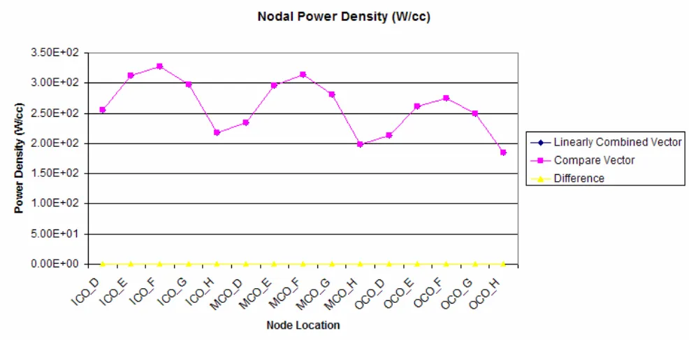
Figure 7: Linearity Test C: Normalized Node Reaction Rate vs. Scaling Factor at EOC 42 Figure 8: Nodal Power Density in Active Core Region ... 46

Figure 9: Covariance Matrices Cx and Cy Singular Value Spectrum vs. Index... 48

Figure 10: Unperturbed Reaction Rate Data vs. Ordered Nodal Location ... 51

Figure 11: Relative Reaction Rate Uncertainty vs. Ordered Nodal Location... 52

Figure 12: Absolute Reaction Rate Uncertainty vs. Ordered Node Location... 53

Figure 13: 15-Group Relative Cross-Section Uncertainty Data ... 57

Figure 14: 15-Group Absolute Cross-Section Uncertainty Data ... 58

Figure 15: Fuel Assembly/Fuel Pin Schematic... 63

Figure 16: B-10 Total Absorption Cross-Section ... 74

Figure 17: C-12 Radiative Capture Cross-Section... 75

Figure 18: Na-23 Total Absorption Cross-Section ... 76

Figure 19: Cr-52 Total Absorption Cross-Section... 77

Figure 20: Mn-55 Total Absorption Cross-Section ... 78

Figure 21: Fe-56 Total Absorption Cross-Section... 79

Figure 22: Ni-58 Total Absorption Cross-Section... 80

Figure 23: Mo-100 Total Absorption Cross-Section ... 81

Figure 24: Inner-Core Neutron Flux Spectrum... 83

Figure 25: Middle-Core Neutron Flux Spectrum... 84

viii

List of Tables

Table 1: TRU Isotopic Composition (%)... 13

Table 2: (U-TRU-Zr) HM/TRU Inventory and Mass Flow Rate ... 15

Table 3: Cross-Section Perturbation Limit ... 43

Table 4: Combined Linearity Test: Perturbed keff Data at EOC... 45

Table 5: Fast Reactor Nominal Values ... 59

Table 6: Key Core Attribute Uncertainties ... 61

Table 7: Key Cross-Section Uncertainty ... 65

Table 8: 15-Group Energy Range ... 66

Nomenclature

Acronyms:

ABTR Advanced Burner Test Reactor BOC Beginning Of Cycle

DC Design Basis Core Simulator DOF Degrees Of Freedom

EFPD Effective Full Power Day ENDF Evaluated Nuclear Data File

EOC End Of Cycle

ESM Efficient Subspace Methods HFP Hot Full Power

HM Heavy Metal

I/O Input/Output Data Stream

LWR Light Water Reactor

LWR-SF Light Water Reactor-Spent Fuel MT Metric-Tonnes

MWD Mega-Watt-Day

PDF Probability Density Function RMS Root Mean Square

SVD Singular Value Decomposition TRU Transuranic(s)

x

1

Introduction

1.1

Purpose

Since the emergence of nuclear power generation, designers have worked to build nuclear reactors that are safe, reliable and efficient. Today, research and development is highly focused on areas pertinent to advanced reactor design systems. The U.S.

will be confined to the development and utilization of an UQ algorithm in support of the research goals listed above.

1.2

Core Simulator Background

The operation of advanced nuclear reactors will place more stringent requirements on the acceptable accuracy of core simulation tools used in support of design and

operation. Core simulators enable designers to model reactor operation, performance, and safety before the expensive construction of the plant takes place. Quantification and understanding of simulators’ uncertainties also allow designers the freedom to change design to reduce design margins which greatly affect operational cost and profit. In addition, with the introduction of advanced reactor systems, i.e. Generation IV reactor systems, the accuracy of the simulation tools needs to be assessed in regard to key core attributes such as decay heat, peak fast fluence, discharge burnup, coolant void worth, etc since the experience with light water reactors (LWR) will not provide an informed basis for assessment due to the large difference in irradiation environment. It is the purpose of this study to use the method of uncertainty quantification to calculate uncertainties found in key core attributes for an advanced reactor system due to cross-sections uncertainties.

1.3

Uncertainty Quantification

cross-section data represents the bulk of input data to core simulation tools, and will be the focus of this UQ study. UQ of key core attributes will provide guidance to models and/or data where further development and/or measurements should be prioritized to reduce attributes uncertainties. Sensitivity and uncertainty analysis of calculated uncertainty estimates is vital in safety analysis, since the reliability of the predictions must be known in order to set realistic design margins for reactor systems; and further reduces the reliance on over-conservatism in design. The target is that by identifying key uncertain cross-sections to which the response is most sensitive, one will be able to improve the cross-sections database used in the analysis and thereby improve the accuracy of the calculations [15].

This thesis presents a recent development of an UQ algorithm for increasing the efficiency of UQ to a level that enables its execution on a routine basis with best estimate calculations for various reactor performance attributes, which denote important reactor core responses. The objective is to devise an algorithm that can characterize uncertainties in the multitudes of reactor performance attributes as evaluated by reactor simulation tools. Some of these attributes include the three-dimensional power and fluence

Our proposed approach reduces the number of model evaluations via the utilization of the Efficient Subspace Methods (ESMs) [3]. ESM is primarily used to perform uncertainty and sensitivity analysis for applications that contain large (I/O) data streams while minimizing the number of required model evaluations. The use of the ESM method has been proven very useful in thermal reactor UQ calculations and has shown that cross-sections uncertainties present a major source of error in thermal reactor calculations [4]. This thesis extends the applicability of ESM to advanced reactor design concepts, specifically sodium cooled fast reactors.

1.4

Uncertainty Quantification Techniques

There are many different types of data originated UQ techniques that have been developed over the years, and a few key techniques are noted below. These techniques include a deterministic and stochastic forward model approach, an adjoint model

approach, and a subspace approach which was ultimately used for this study. However, performing uncertainty calculations can be challenging due to large input/output data streams that are associated with reactor system modeling tools. Uncertainties also arise from numerical discretization approximations and homogenization theory modeling approximations along with finite arithmetic round-off error. For this study, numerical and modeling errors will be neglected and only uncertainties due to cross-sections will be investigated.

1.4.1 Deterministic Forward Technique

varying selected input data one at a time in order to observe an output response. By observing how the output changes via input data perturbation, sensitivity information can be drawn about the perturbed input data. Repeating this methodology over a range of input parameters constructs a sensitivity operator which is used in many sensitivity and uncertainty analyses. This method can be used to propagate uncertainties in models’ input data [14]. Let the matrix denote an input data covariance-variance matrix. Additionally, let us denote as a response and a sensitivity operator where the ith element of is defined by:

C

R S

S

[ ]

_i

i

α

∂ =

∂ R

S . (1.4-1)

Eq. (1.4-1) shows that the sensitivity operator is merely the change in response to some input parameter, α_i. One can show that the response uncertainty, in units of variance, is

given by:

var( )_R =_SCST_{, (1.4-2)} where the variance of the response is calculated by “sandwiching” the input data

covariance matrix between the conformable forms of the sensitivity operator – this relation is often called ‘the sandwich equation’. Even though this method works, calculating the sensitivity matrix and performing the mathematical operation shown in Eq. (1.4-2) is very time consuming and will not be feasible with models that have large amounts of input data.

1.4.2 Adjoint Technique

highlight of the adjoint methodology is that sensitivity coefficients can be calculated for a particular response due to all input data. An ideal setting for this method occurs when there are comparatively fewer responses, , than input parameters,n, i.e. where . Typically, sensitivity coefficients are calculated for selected core responses, thus a

sensitivity matrix for each response pertaining to all input data can be created. As seen in the work by G. Aliberti, et al., a core attribute covariance matrix can be determined by multiplying the sensitivity matrix by the input data covariance matrix, and finally by the transposed sensitivity matrix [11]. Additionally, the adjoint method in Aliberti’s study was used to calculate uncertainties in reactor and fuel cycle parameters in regard to cross-section perturbation [11],[13]. However, sensitivity analysis by adjoint methodology can become time consuming when the number of responses is large, which occurs often in reactor calculations.

m m n<

1.4.3 Stochastic Forward Technique

Another forward technique is known as stochastic sensitivity analysis. This approach works for systems that have larger input and output data streams [14], which is more appropriate for this study. Further, this method uses Monte Carlo sampling

Observing the output after running such input data through computational models allows one to check the distribution in post processing analysis. A great benefit of Monte Carlo sampling is its randomness, which creates an unbiased approach in regards to data sampling. In other words, all data that exists within the input data space has an equal opportunity of being sampled, whereas a biased approach would disregard certain data to help shape output quantities in a particular fashion.

1.4.4 Subspace Technique

ESM is primarily used to perform S/U analysis for applications that contain large (I/O) data streams while minimizing the number of required model evaluations. Such an application is Multi-Scale/Multi-Physics (MSMP) modeling. “Recently, MSMP

1.5

Computational Modeling Description

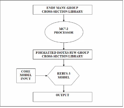
Reactor system modeling is a tool that is utilized in all segments of the nuclear industry for reactor design, optimization and safety. These models map neutronic interaction with various isotopes to simulate core power, flux spectra, depletion characteristics, etc. Generally, a many-group cross-section library that exists for all isotopes in the model must be utilized. For computational storage and run-time

efficiencies, these many-group section libraries are collapsed to few-group cross-section libraries via a processor that performs a lattice physics or pin-cell calculation using flux-averaging and resonance treatment techniques. A core simulator model utilizes the few-group cross-section library and calculates many core attributes.

Figure 1: Black Box Modeling Flow Diagram

Section 1.5.1 and section 1.5.2 describe in detail the MC2-2 processor and REBUS-3 model used in this study, respectively.

1.5.1 MC2-2 Description

The spectrum that is calculated by MC2-2 is used to collapse multi-group to few-group neutron cross-section data. Eq. (1.5-1) presents the general formulation used to calculate macroscopic few-group cross-sections via flux weighting techniques.

( ) ( )

( )

1 1 g g g g g E x E x E E

dE E E

dE E φ φ − − Σ Σ =

∫

∫

K (1.5-1)

where Σx

K

is the effective macroscopic cross-section over selected energy groups,

1

g g

E < <E E ₋ , which is weighted by the group dependent neutron flux. MC2-2

accommodates high-order P scattering representations and provides numerous

capabilities such as delayed neutron processing, isotope mixing, free-format input, and flexibility in output data selection. A fundamental mode homogeneous unit cell calculation is performed using a multi-group or a continuous slowing-down treatment. Multi-group neutron homogeneous cross-sections are then finally generated into an ISOTXS format for an arbitrary group structure [5].

1.5.2 REBUS-3 Description

REBUS-3, here forth denoted as REBUS, is a code system that is designed for the analysis of fast reactor fuel cycles. Much like MC2-2, REBUS was created by ANL and distributed by the RSICC which is located at ORNL. “Two basic types of analysis problems are solved: 1) the infinite-time, or equilibrium, conditions of a reactor operating under a fixed fuel management scheme, or 2) the explicit cycle-by-cycle, or

non-equilibrium operation of a reactor under a specified periodic or non-periodic fuel

length and fuel management scheme. REBUS is also a deterministic core model. Finally REBUS is equipped to model hexagonal-z geometry fuel assembly arrays, which is the design for this study.

2

ABTR Description

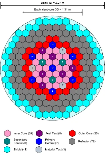
An Advanced Burner Test Reactor (ABTR) was chosen for this study, which is based on a General Electric Hitachi Nuclear’s S-PRISM (SuperPRISM) Fast Reactor Design. S-PRISM is a pool-type, modular design for a sodium-cooled fast reactor designed to operate near breakeven or as a breeder reactor [1]. The ABTR core model is a 250MWt/96MWe liquid sodium-cooled fast reactor that consists of 199 hexagonally shaped assemblies. A breakdown of these assemblies are as follows: 54 driver

assemblies, 78 reflector assemblies, 48 shield assemblies, 10 control rod assemblies and 9 test assemblies, where 6 of these test assemblies are referred as middle-core assemblies in this thesis. The 54 driver assemblies are divided into two enrichment zones, denoted as an inner and outer core region; 24 inner-core fuel assemblies with a TRU fuel enrichment of 16.5% and 30 outer-core fuel assemblies with a TRU fuel enrichment of 20.7%. A ternary metal alloy fuel for the 54 driver assemblies was chosen to be (U-TRU-10Zr) with a 94.2% fissile content WG-Pu feed. The 6 test assemblies, or middle-core

Table 1: TRU Isotopic Composition (%)

Figure 2: ABTR Core Configuration

Table 2 shows the inventory makeup along with mass flow rates for the U-TRU-Zr fuel.

Table 2: (U-TRU-Zr) HM/TRU Inventory and Mass Flow Rate

In Table 2, U238 and Pu239 are the key isotopes that contribute the highest inventory for this core design. U238 contributes 81.68% of HM inventory while Pu239 makes up 85.87% of TRU loading. Pu239 is created via a neutron capture reaction with U238, which creates U239 _{and further decays into Np}239 _{and finally Pu}239_{. Per cycle, two inner and two outer}

fuel drivers are required and Table 2 verifies that U238 and Pu239 are charged and discharged from the core at much higher mass flow rate in comparison to other HM isotopes.

burnup of 97.7/130.8 MWd/kg and a fissile/TRU conversion ratio of 0.58/0.65.

Reactivity control and neutronic shutdown are provided from the use of 7 primary and 3 secondary control assemblies via bank movement mechanisms. The shutdown margin for the primary system, assuming that the most reactive assembly is stuck out, is 7.63$ at BOEC and 12.88$ at EOEC [2].

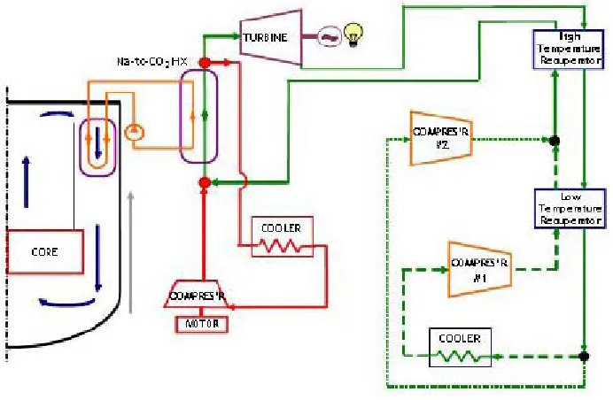
The primary cooling system consists of a pool-type arrangement of liquid sodium that is connected to an intermediate sodium loop. A supercritical CO2 Brayton Cycle

power generation cycle was proposed for this study. A plot of the overall thermodynamic cycle for this proposed ABTR design can be seen in Figure 3.

Figure 3: ABTR Thermodynamic Cycle

As seen in Figure 3, the intermediate sodium loop connects to the supercritical CO2

Brayton Cycle by the means of a Na-to-CO2 heat exchanger where heated CO2 flows into

3

Methodology

The proposed approach is based on the use of the Efficient Subspace Method (ESM), which derives its power from the following three assumptions: A) local linearity of the computational model within range of input data uncertainties, B) ill-conditioning of the covariance matrix characterizing input data uncertainty information, and C) ill-conditioning of the model sensitivity matrix. If condition A is not satisfied, the estimated uncertainties will be only first-order accurate. Conditions B and C are not necessary; however, they correlate the UQ-associated calculational overhead to the degree of ill-conditioning of the input data covariance and model sensitivity matrices.

3.1

Model Local Linearity

Model local linearity is an important aspect that must be taken into account so that key core attribute uncertainties are calculated correctly and that the ESM method can be utilized. As mentioned previously, a fast reactor fuel cycle model (REBUS) was selected to model the ABTR core for a converted equilibrium to non-equilibrium scenario (will be discussed in a later section). REBUS is a non-linear model; however, with the use of local linearity by remaining in range of input data uncertainties, key core response (i.e. attribute) uncertainties can be calculated.

A model that maps ΩK σ ∈ℜK n to _yK∈ℜm _{can be approximated by a local linear}

function around a reference point

(

σK₀,yK₀

)

if it satisfies the following condition:

1

( ) ( ) ( ) ( )

=

′ ⎡ ⎤

ΩK K − ΩK Ko =

∑

k i_⎣ΩK Ki − ΩK K _⎦

i

where and σK yK are vectors characterizing input data and performance attributes, respectively. For the remainder of the paper, we identify variables with single bars as vectors and bold font as matrices. The vector

n m = + K K i o K i

σ σ δσ describes the input data after

being perturbed from their reference values by k random perturbation {δσK_i}. Each

perturbation δσK_i is selected to be linearly independent from all other perturbations.

The

1

k− ′

K

σ is a vector of input data perturbed by a linear combination of the previously selected random perturbations, i.e. k

1 = ′ = +

∑

K K k

o i

i

K

i

σ σ α δσ (3.1-2)

Satisfaction of Eq. (3.1-2) assures linearity of the performance attributes changes with respect to all input data. If some performance attribute exhibits a non-linear relationship with respect to some input data, Eq. (3.1-1) will not be satisfied. The residual of Eq. (3.1-1) can measure the deviation from linear behavior, here denoted by the non-linear error.

This study serves to identify two limits on the sizes { }α_i of input data perturbations: a) an upper limit is selected high enough to ensure that the perturbations cover the ranges of input data uncertainties (i.e. within 4 standard deviations of their respective mean values). This is important to ensure that the computational model behaves linearly with input data varying at the tail ends of their distributions. And b) a lower limit is selected to determine the minimum size of input data perturbations that can induce noticeable changes in performance attributes. These upper and lower cross-section perturbation limits will be found via a prescribed

U

γ

L

numerical tolerance limit,ζ , that is subject to engineering judgment and is determined by the analyst.

To determine the upper limit and lower limit for input data perturbation sizes, two linearity tests were employed. Along with these limits, the linearity tests aid in finding the local linearity region in REBUS for perturbing the input data. There were two techniques used to determine the range, or standard deviation in this case, at which cross-sections could be perturbed and REBUS would remain in a linear region.

U

γ _γL

3.1.1 Scaled Random Cross-Section Perturbation Study

The first technique was to create one random direction, where a direction refers to a certain perturbation of input cross-section data from a reference condition.

Randomness of each section perturbation is important to ensure that all cross-sections will be perturbed without a biased approach. The size of the cross-cross-sections perturbations would then be scaled, using some scaling factor, in that same random direction. Linearity confirms that scaling the input will produce an output perturbation proportional to the size of the scaling factor. By using different scaling factors, the linearity range for REBUS can be found. This linearity method was used to calculate the upper limit, for cross-section perturbation, after exploring several random directions and repeating the scaling procedure described above. The implication is that if the cross-sections perturbations exceed the upper limit then REBUS will behave non-linearly. Based on a prescribed numerical tolerance limit,

U

γ

U

γ

ζ , which varies based upon the reactor system attribute, a maximum cross-section perturbation was found. This follows when:

(

)

( )

(

Ω σo+αδσi − Ω σo

)

−α

(

Ω

(

σo+δσi

)

− Ω

( )

σo

)

>ζ

K _{K K} K _K K _{K K} L _K

where ζ is a prescribed tolerance limit, α denotes the scaled standard deviation, σ_i is the ith perturbed cross-section and σ_o is the reference section. By scaling the

cross-section perturbation vector, one can find when the left-hand side (LHS) of Eq. (3.1-3) becomes greater than the numerical tolerance limit. At this point, the non-linear error exceeds the tolerance limit and thus the upper numerical limit, , for perturbing

cross-sections is found, where

U

γ

U

γ =α.

Furthermore, the numerical tolerance limit was also used to calculate the lower limit , or minimum perturbation for cross-section data that would still produce some noticeable change in modeled output that exist above the non-linear error margin. Similar to finding the upper limit, , calculating the lower limit revolved around some prescribed numerical tolerance limit, denoted as

L

γ

U

γ

ζ . Depending on the attribute, this tolerance limit was based on engineering judgment along with knowledge from thermal reactor analysis [4]. Accordingly, for some random cross-section perturbation direction, a minimum scaling factor was found such that the absolute change in an attribute from running the perturbed and unperturbed cross-sections became less than the numerical tolerance limit, i.e.,

(

σo αδσi

)

( )

σo ζ

ΩK K + K − ΩK K < . (3.1-4)

perturbation, responses will behave linearly due to this cutoff from non-linear error. 3.1.2 Multiple Random Cross-Section Perturbation Study

Although the previous linearity test allowed for the calculation of the upper and lower standard deviation limits, the second test served as a ‘sanity check’ to evaluate the model at these standard deviations where _{σ ⎡γ γ}L, U_⎤

∈ ⎣ ⎦. This technique was to allow a

random number generator to produce random directions. This linearity test differs from the former because this test observes the linearity of n primary directions rather than one. Linearity also shows that if there are n random directions, then a linearly combined case, which is the summation of each random direction multiplied by a random scaling factor can be approximated using a linear model. For this study, it is imperative that the square of scaling factors sum to 1 to ensure that the linearly combined cross-section vector will have the same size as individual cross-section vectors. In equation form, let

[

σ σ1, , ... , 2 σn

]

K K K

denote random cross-section vectors which span from . The

linearly combined cross-section vector is defined below in Eq. (3.1-5),

1...

i= n

1

n

LC o i i

i

σ σ α δ

= = +

∑

σ

K K K _(3.1-5)

where,

( )

2 , _. i i j i RMS n σ σ

σ =

∑

=σK

K K

(3.1-6)

The root mean square (RMS), or quadratic mean, for each individual cross-section vector was set so that L, U

σ

σK_{∈ ⎣}⎡γ γ ⎤⎦, which was set to a conservative 5% in the study.

linearly combined cross-section vector, σK_LC. First, let us introduce the expected value

and variance for a given cross-section vector as E

( )

σK_i =μK_i and

( )

2 i

i

V σK =σ_σK ,

respectively. Taking the first moment or expected value of σK_LC yields:

(

)

1 LC

n

LC o i i

i

E σ μ_σ σ α

= = K = +

∑

μ

K K K K _(3.1-7)

where the expected value of the reference cross-section vector returns itself. Now take the second moment of the variance of σK_LC:

2

(

)

2

LC E LC LC

σ

σK = σK −μK_σK (3.1-8)

where

(

1 1 1

LC

n n n

LC o i i o i i i i i

i i i

σ

)

σ μ σ α σ σ α μ α σ μ = = = ⎛ ⎞ ⎛ ⎞ − =_⎜ + _{⎟ ⎜}− + _⎟= − ⎝

∑

⎠ ⎝

∑

⎠

∑

K

K K K K K K K K

. (3.1-9)

Therefore, the variance of the linearly combined cross-section vector is defined by:

2 2

(

)

2 2

(

)

2

1 1

2 2 1

LC i

n n

i i i i i i i

i i

E E n

i σ σ σ α σ μ α σ μ α σ = = ⎡ ⎤ ⎡ ⎤ =

∑

_⎣ − _⎦=

∑

_⎣ − _⎦=

K K K K K K

=

∑

2

. (3.1-10)

By setting 2 as described above, the following holds. 1 1.0 n i i α = =

∑

2 2 1 LC i n i i σ σ σ α σ = =

∑

K K (3.1-11)

2 2 1 LC n i i

σ σ 2

σ σ α

= =

∑

K K (3.1-12)

σ_σK_LC =σ_σK (3.1-13)

Therefore, Eq. (3.1-13) verifies that the RMS of the linearly combined cross-section vector,

LC

σ

such that _LC L, U

σ σ

σK =σK_{∈ ⎣}⎡γ γ ⎤⎦

)

. Finally, the standard deviation that was chosen, which

exists within the lower and upper limits, can be tested by showing that,

(

)

(

(

)

( )

1

n

i i o LC o

i

y y

α σ σ ζ

=

⎛ ⎞

− − Ω − Ω <

⎜ ⎟

⎝

∑

⎠

K K

K K K K

, (3.1-14)

where α_i are the scaling factors, and yK_i and yK_o denote some ith perturbed and

unperturbed core attribute, respectively.

3.2

Ill-Conditioning of Covariance Data

3.2.1 Theory: Uncertainty Propagation

As seen in uncertainty quantification work by Ronen, the “sandwich rule” is an uncertainty propagation method to calculate a covariance matrix for a set of attributes given:

1) the input parameters covariance matrix

2) and the sensitivity matrix that characterizes the change in attributes per change in input parameters.

Provided with some non-linear computational model which contains input parameter uncertainties described by probability density function (PDFs), the sandwich rule is derived by taking the first and second moments of these corresponding PDFs. In this case, the input parameters uncertainties, i.e. cross-sections uncertainties, are of a

Gaussian distribution. This propagation method ensures that the attributes uncertainties found by calculating the attribute covariance matrix will also have a Gaussian

distribution.

continuous input parameters σK be given by:

E h

( )

σ h

( ) ( )

σ f σ d

+∞

−∞ ⎡ ⎤ =

⎣ K ⎦

∫

K K σK (3.2-1) where E h⎡⎣

( )

σK ⎤⎦ is the expected value of h

( )

σK and f

( )

σK is the PDF that characterizes input parameter uncertainty. Now consider a nuclear reactor core simulator’s non-linear model as a vector valued function:

yK= ΩK( )σK (3.2-2) where yK∈ℜm is a vector of reactor performance attributes, and σ ∈ℜK n _{a vector of}

cross-sections data input to the simulator. Applying Eq. (3.2-1) to the non-linear model shown in Eq. (3.2-2) provides the expected value of yK,

E y

[ ]

( ) ( )

σ f σ σd

+∞

−∞ = Ω

∫

K

K K K K_{. (3.2-3)}

Further, the general definition for the covariance of these attributes is shown below:

COV y y

(

_i, _j

)

=E y_⎢⎡

(

_i−μ_yi

)

(

y_j−μ_yj

)

T⎤_⎥

⎣ K K ⎦

K K K K

, (3.2-4)

where

*

y

μK represents the mean value for the

*

yK attribute [22]. Applying Eq. (3.2-4) to

the non-linear model in Eq. (3.2-2) provides the expected covariance of the attributes,

(

,

)

(

( )

)

(

( )

)

( )

i j

T

i j i y j y

COV y y σ μ σ μ f σ d

+∞

−∞

⎡ ⎤

= _⎢ Ω − Ω − _⎥

⎣ ⎦

∫

K K K K σ

K K K K K K_{. (3.2-5)}

Let us now perform a Taylor series expansion on Eq. (3.2-2). This expansion forms a first-order linear approximation for the non-linear model. Namely,

(

)

( )

2

o o

atσ σK = K_o +uK, where yK is a vector of core attributes, uK represents some cross-section perturbation, is the sensitivity matrix and Ω _O

( )

_Δ2 _{are higher order terms. Further,}

denote yK_Δ = −y yK K_o and σK_Δ = −σ σK K_o for later use. Ideally, the sensitivity matrix can be attained by calculating the adjoint solution which reveals the sensitivity of a core attribute to all input parameters [7]. However, calculating the sensitivity matrix can be very time consuming. By neglecting higher order terms, Eq. (3.2-6) verifies that the sensitivity matrixes effect on a vector can be evaluated by running the non-linear model at two separate points where:

[ ]

( )

1,..., 1,..., i ij j i m for j n σ σ ∂Ω ⎧ = = _{⎨ =} ∂ _⎩ Ω K K

K . (3.2-7)

Substituting the first-order linear approximation of the computational model into Eq. (3.2-3) provides the mean values of the attributes, yK_o, where:

yK_o = ΩK

( )

σK_o . (3.2-8) Notice that the expected value with respect to input parameters is the reference case whereas the expected value of the core attribute yK is simply evaluated by running the model at the input parameters reference case. Finally, let us calculate the first-order approximate covariance for the uncertainties in yK by substituting the first-order linear approximation into the general covariance equation shown in Eq. (3.2-4), where:

(

)

(

(

)

)

(

(

)

)

(

)

(

)

(

(

)

)

(

)

, , T

i j i o j o

T T

i o j o

T

i j

COV y y E

E COV σ σ σ σ σ σ σ σ σ σ ⎡ ⎤ = _⎢ − − _⎥ ⎣ ⎦ ⎡ ⎤ = − − ⎢⎣ = Ω Ω Ω Ω Ω Ω

K K K K K K

K K K K

K K ⎥⎦

In other words, the covariance matrix for core attribute uncertainty is given by:

₌ T (3.2-10)

y x

C ΩC Ω

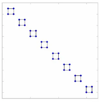
where is a block-diagonal cross-section covariance matrix that was provided by BNL

[6]; each block is 15x15 corresponding to a 15 energy group representation. x

C

Figure 4 presents a graphical interpretation of a block-diagonal matrix.

Figure 4: Block Diagonal Matrix

Let us also point out that any general covariance matrix, i.e. a full matrix without a trend, can be broken down into diagonals and off-diagonals. Mathematically, diagonals of a covariance matrix represent the variance of a particular attribute whereas

off-diagonals represent the correlation between two different attributes. Taking the

covariance of one component with respect to itself yields the variance for that specified component, where:

(

_,

)

2 2

i i

i i i y y

COV y y =E⎡_⎢ y −μ ⎤_⎥=σ

⎣ K ⎦ K

K K K _{. (3.2-11)}

Therefore, the diagonal entries for a given covariance matrix, i.e. the cross-section covariance matrix in this case, are in units of variance and can simply be converted into standard deviation by taking the square root of these diagonal entries.

Conventionally, uncertainty analyses attempt to create the sensitivity matrix in order to calculate the core attribute covariance matrix shown in Eq. (3.2-10); however, with large amounts of input/output (I/O) streams, using the adjoint method to create a sensitivity matrix is very time consuming and expensive, i.e. responses would require

adjoint solutions. Therefore, a forward model approach which harnesses the strength of ESM was utilized.

m

m

3.2.2 ESM-Based Approach

In using the ESM approach, it is imperative to show how ESM builds a low rank approximation to the sensitivity or Jacobian matrix. The theory behind this approach relates to the Orthogonal Decomposition Theorem, noted in linear algebra work. This theorem shows that for every _Ω∈ℜm x n,

where _σ n and .

Δ∈ℜ

K _y m

Δ∈ℜ

K

n

Further, an orthogonal decomposition of _ℜm and _{ℜ can be computed as follows:}

( )

( )

( )

( )

m _{R R} ⊥ _{R N} T

ℜ = Ω ⊕ Ω = Ω ⊕ Ω (3.2-13)

( )

( )

( )

( )

n _{N N} ⊥ _{N R} T

ℜ = Ω ⊕ Ω = Ω ⊕ Ω (3.2-14) where R

( )

* denotes the range-space, _R

( )

*T _{denotes the row-space, denotes the}

null-space, denotes the left-hand null-space, and

( )

*

N

( )

*T

N ⊕ signifies that are

spaces which contain orthogonal complementary subspaces. Given that ,

the size for each subspace can be written as follows:

and

m n

ℜ ℜ

( )

rank Ω =r_Ω

( )

( )

( )

(

dim dim T dim dim T

r_Ω = R Ω = R Ω = −n N Ω = −m N Ω

)

(3.2-15)

where ‘dim’ stands for the dimension of , or the number of vectors in any maximal independent subset for columns or rows of the sensitivity matrix. Eq. (3.2-15) is significant because it shows the extent of independent data present within these fundamental subspaces. Furthermore, it was shown that

Ω

n

σK_Δ∈ℜ and ; now let’s apply this subspace approach to the linearly approximated model shown in Eq. (3.2-6),

m

yK_Δ∈ℜ

(

)

y σ σ⊥ σ σ

Δ =Ω Δ =Ω Δ + Δ& =Ω &

K K K K

Δ

K _{. (3.2-16)}

Eq. (3.2-16) demonstrates that _σ n

Δ∈ℜ

K _{can be broken down into subspaces where,}

following Eq. (3.2-14), _{σ R}

(

T , therefore

Δ∈ Ω

&

K

₎

_σ⊥ _N

_{( )}

Δ ∈ Ω

K

. The importance of this

modeled output, such that yK_Δ∈R

( )

Ω . Therefore, the action of the sensitivity operator upon input data from N

( )

Ω will map to0K. Hence, data from N

( )

Ω is no longer needed

and from Eq. (3.2-15) it was shown thatdim_R

( )

₌dim_R

( )

T _=r

Ω

Ω Ω . Ultimately, this

reveals that only independent input data perturbations from r_{Ω R}

( )

_ΩT _{are needed to}

change the output of core attributes [9],[19].

3.2.3 Mathematical Method to Calculate CoreAttribute Covariance Matrix As shown in Eq. (3.2-10), is the cross-section covariance matrix that was

provided by BNL. Previous work has illustrated that x

C

x

r , or the rank of , is often much

smaller than the size of the input cross-section data and the output performance attributes, i.e. , implying that only

x

C

x

r n, m r_x forward model evaluations are required to quantify

uncertainties in the attributes yK[9]. The following methodology was used to prove that

the cross-section covariance matrix, , is of a rank deficient form. Start by taking the

singular value decomposition (SVD) of the block-diagonal matrix , which takes the

form: x C x C 2 =

C WΣ WT

x x , (3.2-17)

diag{ } x x

r × r

j

s

=

Σ_x , (3.2-18)

_[

x

1 2 r

w w .... w

× ₌

Wn rx K K K ] (3.2-19)

and { }2 j

s , and { }wj

K _{are the eigenvalues and eigenvectors of the cross-section’s}

equivalent. Matrix contains a set of orthonormal basis vector directions for ,

where each {

W Cx

}

j

wK refers to some direction in the input data space, i.e. a perturbation of all

input data that is uncorrelated with all other perturbations. Finally, the matrix 2

x

Σ

contains the eigenvalues which have units of variance. A cross-section perturbation matrix can now be created which aids as an input to REBUS.

X =Wn x rxAr x rx x, (3.2-20)

r x rx x

{ }

j

diag α

=

A , (3.2-21)

where is the cross-section perturbation matrix, is the left singular vector matrix from the SVD of , and A is a diagonal matrix composed of scalars,

X W

C_x α_j, that fix the

root mean square (RMS) for each column in W to a set standard deviation of σ_xK, or 5%

to ensure that linearity of the REBUS model holds. The dimensions for the cross-section perturbation matrix are , where n represents the total number of isotopes, reaction type, spatial composition and all 15 energy groups. Each column from is now a cross-section perturbation input file that will be run separately in REBUS. Running the perturbation matrix through REBUS produced an output matrix composed of reaction rates, which span all nodes in the core for all isotopes and fission/capture reactions, which took the form shown in Eq. (3.2-22),

x

n x r X

x

n x r X

_Y' =_{ΩX. (3.2-22)}

'

m x rx = ' -1 . (3.2-23) x

Y Y A Σ

Using an ESM-based UQ approach [8], one can show that uncertainties in yK

characterized by a covariance matrix C_y, may be given by:

[ ] [ ]

_* 1 x r T T

y j _*j

j=

= =

∑

C YY Y Y (3.2-24)

where,

[ ]

Y _*j =Ωw sj j = Ω(σ0 +w sj j)− Ω( )σ0

K K

K K K K _{. (3.2-25)}

Eq. (3.2-24) demonstrates how the ESM method provides another route to calculate the core attribute uncertainty covariance matrix without the explicit knowledge of the sensitivity matrix . Matrix Y, or the uncertainty response matrix, shown in Eq. (3.2-25) is formed simply by running the model at two points, namely at some perturbed point along with the unperturbed reference point.

Ω

Notice that the summation in Eq. (3.2-24) runs up to r_x, the numerical rank of the

cross-sections covariance matrix, which is determined via a singular value

decomposition. By observing the decline in the singular values from the SVD of ,

one can utilize the lower limit for cross-section perturbation,

C_x

L

γ , to find a cutoff point at

which certain perturbations contain too small of a magnitude to produce any change in core attribute output. The lower cross-section perturbation limit revealed that

which proves that C is indeed ill-conditioned. Therefore, only

x

r n,m

x rx forward model

3.3

Ill-Conditioning of Model Sensitivity Matrix

m

Another goal of this thesis was to present a recent development of an UQ algorithm for increasing the efficiency of UQ to a level that enables its execution on a routine basis with best estimate calculations for various reactor performance attributes. To accomplish this, the latter part of this study dealt with the investigation of further reducing the

amount of forward model evaluations by examining the ill-conditioned nature of the sensitivity matrix. The sensitivity matrix is a rectangular matrix that contains the first order derivatives of m core attributes with respect to input data. Ill-conditioning of the sensitivity matrix implies that the number of independent input data perturbations leading to changes in attributes is much less than the number of input data and attributes, i.e. the matrix rank: , which was shown in section 3.2.2.

n

Ω

r n,

For this study, this proposed approach reduces the number of model evaluations to a minimum by recognizing that the rank of the covariance matrix of core attributes

is much smaller than the rank of the cross-sections covariance matrix . Again, this is

due to the dimensionality reduction induced by the forward model whose numerical rank is also shown to be very small. Following Eq. (3.2-24), it was shown that the

core attribute covariance matrix could be calculated with

y C x C Ω Ω r x

r model evaluations. It is the

intension of this section to prove that:

[ ] [ ]

_{* * post post post post}

*

1 1

= = *

⎡ ⎤ ⎡ ⎤ =

∑

= = =

∑

_{⎣ ⎦ ⎣ ⎦}

YY Y Y C Y Y Y Y

post x r r T T T T y

j j _{j j}

j j

(3.3-1)

where we can calculate the core attribute covariance matrix by capturing the effect of r_x

shown below, provides the algorithm that was used to calculate the core attribute covariance matrix in a reduced rpost forward model evaluations.

3.3.1 Algorithm to Compute Reduced Core Attribute Covariance Matrix

,r

,r

Studies have shown that is smaller than the effective numerical ranks of

either the sensitivity matrix or the cross-section covariance matrix, i.e. .

This assures that the amount of forward model evaluations to calculate the core attribute covariance matrix can be reduced. With

post

r

min( )

post Ω x

r ≤ r

y

C rpost ≤min(rΩ x) known, a methodology to

reduce forward model evaluations to compute the core attribute uncertainty covariance matrix was created. One can exploit this by first performing an SVD factorization of the uncertainty response matrix in Eq. (3.2-25) as follows: Y

post post x m × r

m × r

post post _* post post _* 1

=

⎡ ⎤ ⎡ ⎤ ⎡ ⎤

=

∑

_{⎣ ⎦ ⎣ ⎦ ⎣ ⎦}

Y Y U Σ V

r

T

j jj j

j

, (3.3-2)

where r_post is the effective rank of the matrix Y_post. The effective numerical rank of

matrix Ypostcan be found by a short algorithm that will be discussed in section 4.2.1. Eq.

(3.3-2) also shows that the SVD of the uncertainty response matrix is equivalent to the SVD of the reduced uncertainty response matrix,

Y

post

Y . Let us now set Eq. (3.3-2) equal

to Eq. (3.2-23), where one can show that:

m x rpost , (3.3-3)

post post post = post =

U Σ VT Y ΩWΣ

x

where the effect of taking the SVD of Ypostis equal to running REBUS with forward

model evaluations. Taking the transpose of

post

r

post T

V on both sides of Eq. (3.3-3) yields a

UpostΣpost =ΩWΣxVpost, (3.3-4)

z_j =WΣx⎡_⎣V_{post *}⎤_{⎦ j}

K _(3.3-5)

where zK_j denotes the linearly combined post-processed cross-section perturbation vector. As mentioned previously, the SVD of a matrix is a type of ordered factorization that orders singular values in a descending order. In this case, the first columns of the

matrix

post

r

post

V form an orthogonal basis for the fundamental subspaceR

( )

Y_post . It was

found that using the first rpost singular vectors, or primary directions, fromVpost, which is

used to linearly combine perturbation vectors in z=⎣⎡z1 ... zj⎤⎦, j=1, rpost

K K _{, can be}

evaluated through REBUS to produce similar data found from r_x forward model

evaluations. Namely, from Eq. (3.2-25) and Eq. (3.3-2), one can re-write Eq. (3.2-24) as:

post

post _* post 1

= *

⎡ ⎤ ⎡ ⎤ ⎣ ⎦ ⎣ ⎦

∑

C = Y Y

r

T

y _{j j}

j

, (3.3-6) where

post * (σ0 zj) (σ0

⎡ ⎤ = Ω + − Ω

⎣Y ⎦ j )

K _{K K} K _K

. (3.3-7)

At this point in the derivation, the core attribute covariance matrix was calculated using reduced r_post forward model evaluations. It is also shown in Eq. (3.3-7) that Y_post was

calculated using the derived linearly combined cross-section perturbation vector from Eq. (3.3-5). Finally, substituting the SVD of Ypost, which is shown in Eq. (3.3-2), into Eq.

(3.3-6) yields an equation that calculates Cy, where

post

post post post _* post post post 1

=

⎡ ⎤ ⎡

⎣ ⎦ ⎣

∑

C = U Σ V V Σ U

r

T

y ⎤⎦_*

T

j j

j

However, computational time associated with the calculation of shown in Eq. (3.3-8)

is high due to the fact that , where

y

C

post

mr m x rpost m x rpost

post post

T

⎡ ⎤ ⎡ ⎤

= ⎣ ⎦ ⎣ ⎦

y

C Y Y . This matrix times

matrix operation requires

{

2

}

{

2

(

1

)

}

post post

m * r + m r − multiplication and addition operations. By realizing the orthogonal nature of V_post, where 1

post post −

=

T

V V , Eq. (3.3-8) simplifies to

post

2

post post _{post *} 1

=

⎡ ⎤

⎣ ⎦

∑

C = U Σ U

r

T

y _j

j

. (3.3-9)

Recall that all input data, denoted by σK, are contained where σ ∈ℜK n_{. Note that the size}

of the input data space is , whereas the sources of uncertainty have been reduced to , i.e. the effective rank of . Therefore, Eq. (3.3-9) shows that core attribute

uncertainties can be calculated via forward model evaluations compared to the

former evaluations by use of the singular vector and singular value matrices,

n

post

r C_y

post

r

x

r <<n

post

U and 2 post

Σ , respectively.

3.4

Uncertainty Quantification

3.4.1 Key Attribute Uncertainties Quantification

At this point in the study, an efficient algorithm which utilizes the ESM

techniques has been completed to calculate the core attribute uncertainty matrix with rpost

reactor work, but increase profits by reducing design margins between operating and limiting parameters via reactor design optimization and experimentation. Such core attributes for the ABTR include discharge burnup, conversion ratios, and power peaking factors, to name a few. These quantities, along with more attributes, will be the primary focus for uncertainty quantification.

Let denote an unperturbed key core attribute that was either calculated or

documented in this study. It was previously found and shown in Eq. (3.3-6) that the core attribute covariance matrix can be calculated in reduced forward model

evaluations. Now set some perturbed response, which exist in

l o

y

y

C r_post

l i

y Y_post, for

where denotes total number of responses. Arbitrarily setting to contain only one

response allows us to generate an equation to calculate core attribute uncertainty. Begin by subtracting then dividing each perturbed response by the nominal value to form a relative quantity:

1,

l= m

m C_y

ˆ l l l i i l o o y y y y − =

, for (3.4-1) 1, 1, post i r l m = ⎧ ⎨ = ⎩

where denotes a relative response for run ‘i’ and response ‘l’. Applying the same

principles used in Eq. (3.2-23), the linearity normalization factors from matrix that were used in pre-processing work,

ˆl i

y

A

α, must be taken out to accurately calculate any uncertainty, i.e., ˆ * l l l i i l o i o y y y y α − =

Given that has been arbitrarily set to contain one response, Eq. (3.3-6) is now a

vector-row multiplied by vector-column operation. In linear algebra terms, this equates to the squared Euclidean norm which can be seen in Eq. (3.4-3),

y

C

( )

2 post post 1 2 2 ˆ 1 * post post l r T l i i

r l l

i o

l y

i i i

y y y y σ α = = = ⎛ − ⎞ ⇒ = _{⎜ ⎟} ⎝ ⎠

∑

∑

Y Y

. (3.4-3)

Therefore, the uncertainty for any key core attribute was found by taking the square root of Eq. (3.4.3):

2 ˆ 1 * post l

r l l

i o

l y

i i i

y y y σ α = ⎛ − ⎞ = _⎜ ⎝ ⎠

∑

⎟ . (3.4-4)

3.4.2 Identification of Key Uncertain Cross-Sections

As mentioned in the introduction to this thesis, one goal of this study was to identify the key isotopes/reaction type combination that contributed the most to these calculated uncertainties. By taking the forward model approach, a single input parameter can be perturbed which in turn affects all output data. Hence, this method allows one to pinpoint key input data that contributes to higher core attribute uncertainty. Recall that Eq. (3.2-17) presents the SVD of the block-diagonal cross-section covariance matrix ,

where matrices that contain the eigenvalues and eigenvectors for C are presented in Eq. (3.2-18) and Eq. (3.2-19), respectively. Additionally, these eigenvalues correspond to isotopes with specific reaction types that exist in a range of energy groups. One can show that these eigenvalues represent an uncertainty for each isotope/reaction rate combination.

C_x

Furthermore, a methodology, described below, which harnesses the standard deviation of diagonal entries from the cross-section covariance matrix, was used to identify the important cross-sections that contribute to high core attribute uncertainty. Taking the SVD of the uncertainty response matrix in Eq. (3.2-23) reveals a similar form seen in Eq. (3.3-1) with the reduced evaluations. The importance of

this factorization lies with the right-hand singular vector matrix which is composed of

x

m x r Y

post

r

V

post

r orthonormal column vectors. Due to the factorization techniques of the SVD, higher

level importance vectors are placed from left to right in . Therefore, by ordering the first column in from high to low, the corresponding singular values can also be ordered with the same index. Thus, this technique provides a descending ordered list of isotopes with specific reaction types that exist at a certain energy group with

corresponding uncertainty values.

4

Results

4.1

Model Linearity

Before utilizing this ESM based methodology for uncertainty quantification of key core attributes for this ABTR design, a linearity study was performed on a non-linear fast reactor fuel cycle model. Recall from section 3.1 that the ESM method can be employed assuming that the computational model behaves linearly within range of input data uncertainties; two linearity studies were presented in section 3.1 to ensure that. 4.1.1 Scaled Random Cross-Section Perturbation Study

The first linearity test consists of scaling the cross-section perturbations vectors, which are randomly generated, by factors ranging from zero, denoting no cross-section perturbation, to five times their initial standard deviation, set to be 5% for all

perturbations vectors. By plotting core attribute deviations from the unperturbed case one can determine if the model behaves linearly with cross-sections perturbations. For this linearity study, two core attributes were selected, the multiplication factor, and reaction rates. The multiplication factor k_eff is defined by:

Number of neutrons in generation (n) Number of neutrons in generation (n-1)

eff

k ≡ , (4.1-1)

also referred to as core reactivity; the multiplication factor is a global reactor

performance metric that describes the balance of neutrons, a core reactivity of 1.0 implies that neutrons are produced and lost at the same rate thus ensuring a self-sustained

at the end of cycle, i.e. [Perturbed-DC] data collected for this study. Let ‘DC’ denote the unperturbed case.

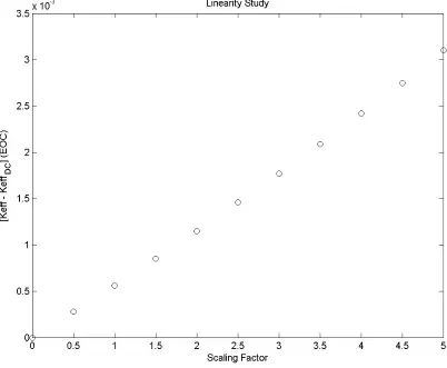
Figure 5: Linearity Test A: Normalized keff vs. Scaling Factor at EOC

It is evident from Figure 5 that as the standard deviation is scaled from

[ ]

0,5 the absolute change in taken at EOC increases linearly. To create an unbiased approach to

cross-section perturbation, multiple randomly generated vectors were employed to repeat the previous study and model local linearity was observed.

eff

k

Figure 6: Linearity Test B: Normalized keff vs. Scaling Factor at EOC

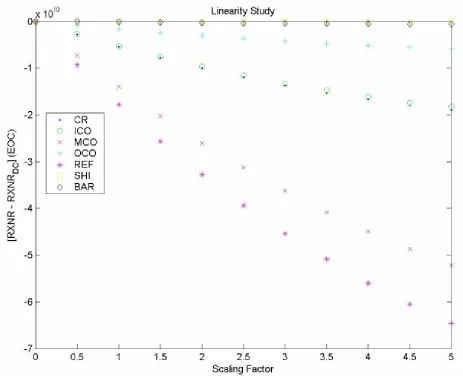
Figure 7: Linearity Test C: Normalized Node Reaction Rate vs. Scaling Factor at EOC

representation. Therefore, the linearity of all reaction rates was confirmed and only a few reaction rates were arbitrarily chosen to represent each core region.

After conducting these linearity tests with different random directions, the lower and upper limits for cross-section perturbation could be found via the use of the

prescribed numerical tolerance limit. Based on thermal reactor analysis experience [4], the numerical tolerance limit was set to 10 pcm and 0.1% for reactivity and core power density, respectively. Table 3 shows the results for the lower and upper cross-section perturbation limits.

Table 3: Cross-Section Perturbation Limit Cross-Section Perturbation Limit (Standard Deviation)

Lower Limit - _γL _{Upper Limit - γ}U

0.01% 7.50%