ABSTRACT
DAWN, WILLIAM CHRISTOPHER. Simulation of Fast Reactors with the Finite Element Method and Multiphysics Models. (Under the direction of Scott P. Palmtag).
Renewed interest in advanced nuclear power reactors, such as the Versatile Test Reactor (VTR) at
Idaho National Laboratory (INL), has encouraged enhanced modeling and simulation of fast nuclear power reactors. Since the inception of fast reactors in the early days of nuclear engineering, with reactors
such as at the Experimental Breeder Reactor I (EBR-I) and Fermi 1, many new modeling techniques
have been developed. This work seeks to introduce modern methods and multiphysics simulation of fast reactors.
In this work, the multigroup neutron diffusion equation is solved via the Finite Element Method
(FEM), allowing for the use of unstructured and general meshes. By using an unstructured mesh, physical phenomena such as thermal expansion can be modeled and allowed to distort the mesh. Additionally,
the FEM will allow for spatial refinement by means of both traditional mesh refinement and the use of higher-order methods without regenerating the mesh. Unique to this thesis is the use of pentahedral wedge
elements in the FEM mesh for three-dimension simulations. Wedge elements are selected for their natural
description of hexagonal geometry common to fast reactors.
Thermal feedback effects within a fast reactors are also modeled in this work. A simplified thermal
hy-draulic model is developed, modeling both axial heat convection and radial heat conduction. Temperatures
from this model are used to calculate temperature dependent neutron cross-sections. In addition to the thermal hydraulic model, a thermal expansion model is developed. Thermal expansion effects significantly
impact reactor behavior and contribute to the passive safety of fast reactor designs as demonstrated in the
experiments performed at Experimental Breeder Reactor II (EBR-II) [Pla87].
Using the multiphysics models developed in this work, a typical fast reactor is simulated at operating
conditions. The models as implemented demonstrate expected reactor behavior for a fast reactor. For the
simulated reactor, reactivity feedback coefficients are calculated which would not be possible without a coupled multiphysics model. These results can be used to describe the passive safety features and
© Copyright 2019 by William Christopher Dawn
Simulation of Fast Reactors with the Finite Element Method and Multiphysics Models
by
William Christopher Dawn
A thesis submitted to the Graduate Faculty of North Carolina State University
in partial fulfillment of the requirements for the Degree of
Master of Science
Nuclear Engineering
Raleigh, North Carolina
2019
APPROVED BY:
Joseph M. Doster Ralph C. Smith
DEDICATION
BIOGRAPHY
William Christopher Dawn was born and raised in Stafford, Virginia. He attended public schools there for his primary education, participating in the Commonwealth Governor’s School in High School. William
earned a Bachelor’s of Science degree in Nuclear Engineering from North Carolina State University (NC
State) in May 2017. After his Master’s degree, William will remain at NC State to pursue a Ph.D. degree in Nuclear Engineering.
William is a fellow of the Integrated University Program (IUP) facilitated by U.S. Department of
Energy Office of Nuclear Energy (DOE-NE). During his undergraduate and graduate careers, he has had the opportunity to work with GE-Hitachi Nuclear Energy Americas LLC (GEH) and Oak Ridge National
Laboratory (ORNL). William has also made contributions to the Consortium for Advanced Simulation of
ACKNOWLEDGEMENTS
This work would not have been possible without the help of friends and family. I would like to thank my Mom and Dad, Suzanne and Bill Dawn, for their patience, their listening, and their advice. Their support
has helped to make this work a reality.
I would also like to thank my advisor, Dr. Scott Palmtag. We have both learned tremendously during this process. His consistency and desire to know more have kept me busy these last few months and I am
TABLE OF CONTENTS
List of Tables . . . viii
List of Figures . . . x
List of Acronyms . . . xii
Chapter 1 Introduction . . . 1
1.1 Motivation . . . 1
1.2 Geometry Description . . . 2
1.3 Cross Section Treatment . . . 5
1.4 Thesis Organization . . . 7
Chapter 2 Finite Element Neutron Diffusion . . . 9
2.1 Introduction . . . 9
2.2 Multigroup Neutron Diffusion Equation . . . 10
2.3 Formulation of Finite Element Equations . . . 12
2.3.1 Derivation . . . 12
2.3.2 Matrix Quantities . . . 17
2.3.3 Quadratures . . . 22
2.4 Power Iterations . . . 24
2.4.1 Convergence of Power Iteration Method . . . 25
2.4.2 Calculation of Source with Power Iterations . . . 28
2.5 Implementation . . . 28
2.5.1 Algorithm . . . 29
2.5.2 Memory and Storage . . . 31
2.5.3 Boundary Conditions . . . 32
2.5.4 Linear System Solution . . . 33
Chapter 3 Neutron Diffusion Results . . . 36
3.1 Introduction . . . 36
3.2 Error Analysis . . . 37
3.3 Analytic Solutions . . . 38
3.3.1 One-Dimension, One-Group, Fixed Source . . . 38
3.3.2 One-Dimension, One-Group, Criticality . . . 38
3.3.3 Two-Dimension, One-Group, Criticality . . . 40
3.3.4 One-Dimension, Two-Group, Criticality . . . 40
3.3.5 One-Dimension, One-Group, Two-Region, Criticality . . . 40
3.3.6 Three-Dimension, One-Group, Finite Cylinder . . . 40
3.4 Two-Dimensional Benchmark Solutions . . . 43
3.4.1 VVER440 . . . 43
3.4.2 SNR . . . 45
3.4.3 HWR . . . 46
3.5 Three-Dimensional Benchmark Solutions . . . 50
3.5.1 MONJU . . . 50
3.5.2 KNK . . . 51
Chapter 4 Thermal Hydraulics . . . 52
4.1 Introduction . . . 52
4.2 Material Properties . . . 52
4.3 Power Normalization . . . 54
4.4 Axial Convection Model . . . 55
4.4.1 Geometric Model . . . 55
4.4.2 Channel Mass Flow . . . 57
4.4.3 Chunk Powers . . . 57
4.4.4 Channel Enthalpy . . . 57
4.5 Radial Conduction Model . . . 58
4.5.1 Geometric Model . . . 59
4.5.2 Surface Temperature and Centerline Temperatures . . . 59
4.5.3 Average Temperatures . . . 67
4.6 Cross Section Treatment . . . 69
4.6.1 Coolant Cross Sections . . . 71
4.6.2 Clad Cross Sections . . . 71
4.6.3 Bond Cross Sections . . . 71
4.6.4 Fuel Cross Sections . . . 72
4.7 Thermal Hydraulic Results . . . 72
4.7.1 Total Reactor Power . . . 72
4.7.2 Radial Results . . . 73
4.7.3 Axial Results . . . 74
Chapter 5 Thermal Expansion . . . 78
5.1 Necessity of Modeling . . . 78
5.2 Material Properties . . . 79
5.3 Model Details . . . 80
5.3.1 Expansion of Finite Element Coordinates . . . 81
5.3.2 Expansion of Area Fractions . . . 83
5.3.3 Conservation of Material and Cross Section Effects . . . 83
5.4 Results . . . 85
Chapter 6 Coupled Multiphysics Results . . . 87
6.1 Power Reactor Modeling . . . 87
6.2 Advanced Burner Reactor – MET-1000 . . . 87
6.3 Reactivity Coefficients . . . 90
6.3.1 Power Reactivity Coefficient . . . 91
6.3.2 Thermal Expansion Reactivity Coefficient . . . 91
6.3.3 Fuel Temperature Reactivity Coefficient . . . 92
6.3.4 Coolant Temperature Coefficient . . . 92
Chapter 7 Summary, Conclusions, and Recommendations . . . 96
7.1 Summary of Simulation Results . . . 96
7.2 Conclusions . . . 97
7.3 Recommendations for Future Research . . . 97
7.3.1 Depletion Capabilities . . . 98
7.3.2 Higher Order Finite Elements . . . 98
7.3.3 SimplifiedPN Solution . . . 98
7.3.4 Encouraging Code Usage . . . 98
Bibliography . . . 100
Appendices . . . 103
Appendix A Analytic Solutions to the Neutron Diffusion Equation . . . 104
A.1 Introduction . . . 104
A.2 One-Dimension, One-Group, Fixed Source . . . 106
A.3 One-Dimension, One-Group, Criticality . . . 108
A.4 Two-Dimension, One-Group, Criticality . . . 111
A.5 One-Dimension, Two-Group, Criticality . . . 114
A.6 One-Dimension, One-Group, Two-Region, Criticality . . . 118
A.7 Finite-Cylinder, One-Group, Criticality . . . 124
Appendix B Brief Compendium of Neutron Diffusion Benchmarks . . . 130
B.1 Introduction . . . 130
B.2 Two-Dimensional Benchmark Problems . . . 131
B.2.1 VVER440 . . . 132
B.2.2 SNR . . . 133
B.2.3 HWR . . . 136
B.2.4 IAEA Hex . . . 136
B.3 Three-Dimensional Benchmark Problems . . . 140
B.3.1 MONJU . . . 141
LIST OF TABLES
Table 1.1 Temperatures Selected for Cross Section Libraries. . . 6
Table 2.1 Quadrature Orders for FEM Quantities. . . 23
Table 2.2 Jacobi for Selected Elements. . . 23
Table 3.1 One-Dimension, One-Group, Fixed Source Convergence Study Results. . . 39
Table 3.2 One-Dimension, One-Group, Criticality Convergence Study Results. . . 39
Table 3.3 Two-Dimension, One-Group, Criticality Convergence Study Results. . . 40
Table 3.4 One-Dimension, Two-Group, Criticality Convergence Study Results. . . 41
Table 3.5 One-Dimension, One-Group, Two-Region, Criticality Convergence Study Results. 41 Table 3.6 Finite Cylinder Convergence Study Results. . . 43
Table 3.7 VVER440 Benchmark Convergence Study. . . 44
Table 3.8 SNR Benchmark Convergence Study. . . 46
Table 3.9 HWR Benchmark Convergence Study. . . 46
Table 3.10 IAEA Hex Benchmark Convergence Study. No Reflector.α=0.125. . . 48
Table 3.11 IAEA Hex Benchmark Convergence Study. No Reflector.α=0.500. . . 48
Table 3.12 IAEA Hex Benchmark Convergence Study. With Reflector.α=0.125. . . 49
Table 3.13 IAEA Hex Benchmark Convergence Study. With Reflector.α=0.500. . . 49
Table 3.14 MONJU Benchmark Rod Worth Results. . . 50
Table 3.15 KNK Benchmark Rod Worth Results. . . 51
Table 4.1 Default Constant Thermal Conductivity for Sodium and HT9. . . 53
Table 4.2 System Properties for Axial Model Verification. . . 74
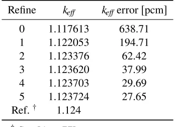
Table 6.1 Advanced Burner Reactor Refinement Results. . . 88
Table 6.2 Multiphysics Contributions to Total Power Defect. . . 94
Table A.1 Case Matrix for Analytic Solutions. . . 105
Table A.2 One-Group Sample Cross Sections. . . 110
Table A.3 Two-Group VVER440 Material Constants. . . 118
Table A.4 Two-Region Material Constants. . . 123
Table A.5 Finite Cylinder Cross Sections. . . 128
Table B.1 Case Matrix for Benchmark Solutions. . . 131
Table B.2 VVER440 Cross Sections. . . 133
Table B.3 VVER440 Fission Spectrum. . . 133
Table B.4 SNR Cross Sections. . . 135
Table B.5 SNR Fission Spectrum. . . 136
Table B.6 HWR Cross Sections. . . 138
Table B.7 HWR Fission Spectrum. . . 138
Table B.8 IAEA Hex Effective Neutron Multiplication Factors. . . 138
Table B.9 IAEA Hex Cross Sections. . . 140
Table B.11 MONJU Effective Neutron Multiplication Factors and Rod Worths. . . 141
Table B.12 MONJU Cross Sections. . . 143
Table B.13 MONJU Fission Spectrum. . . 143
Table B.14 KNK Effective Neutron Multiplication Factors and Rod Worths. . . 144
Table B.15 KNK Cross Sections (Part A). . . 147
Table B.16 KNK Cross Sections (Part B). . . 148
LIST OF FIGURES
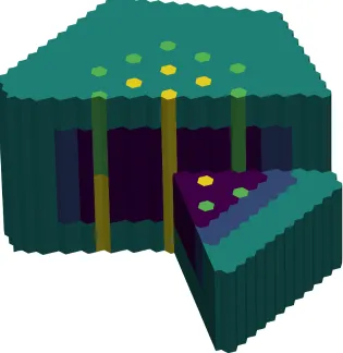
Figure 1.1 Example of Fast Reactor Materials based on MONJU. . . 3
Figure 1.2 Example of Fast Reactor Fuel Assembly Cross Section. . . 3
Figure 1.3 Dimensions of Thermal Hydraulic Rod Model (not to scale). . . 4
Figure 1.4 Dimensions of Hexagonal Can (not to scale). . . 5
Figure 2.1 Example of Rectangular Unstructured Mesh. . . 13
Figure 2.2 Description of Triangle Elements. . . 18
Figure 2.3 Description of Wedge Elements. . . 20
Figure 2.4 Description of Reference Wedge. . . 21
Figure 2.5 Typical Fast Flux Visualization for Two-Dimensional and Three-Dimensional Simulations. . . 29
Figure 2.6 Demonstration of RCM Matrix Ordering. . . 30
Figure 2.7 Example Unstructured Mesh. . . 32
Figure 3.1 Mesh Refinement of Curved Mesh. . . 42
Figure 3.2 VVER440 Benchmark Power Comparison for Most Refined Mesh. . . 44
Figure 3.3 SNR Benchmark Power Comparison for Most Refined Mesh. . . 45
Figure 3.4 HWR Benchmark Power Comparison for Most Refined Mesh. . . 47
Figure 4.1 Variable Thermal Conductivity in Fuel. . . 54
Figure 4.2 Progression of Element, to Chunk, to Channel. . . 56
Figure 4.3 One-Dimensional Axial Heat Convection Model Description. . . 56
Figure 4.4 Geometry Description of Radial Heat Conduction Model (not to scale). . . 59
Figure 4.5 Radial Temperatures for Typical Fuel Rod. . . 73
Figure 4.6 Difference Between Analytic and Modeled Axial Temperatures for 36 Axial Levels. 76 Figure 4.7 Average Axial Temperatures for Model Reactor Conditions. . . 77
Figure 5.1 Linear Expansion Factor for HT9 Steel and U10Zr Fuel. . . 80
Figure 5.2 Thermal Expansion of General Volume. . . 82
Figure 5.3 Effective Neutron Multiplication Factor as a Function of Thermal Expansion Temperature. . . 86
Figure 5.4 Reactivity as a Function of Thermal Expansion Temperature. . . 86
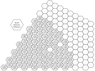
Figure 6.1 Materials in ABR. . . 89
Figure 6.2 Fast and Thermal Neutron Flux in ABR. . . 90
Figure 6.3 Feedback Effects onkeff. . . 94
Figure 6.4 Advanced Burner Reactor (ABR) Reactivity Coefficients. . . 95
Figure A.1 Fixed Source and Criticality Flux Shapes for One-Dimension, One-Group Problems.108 Figure A.2 Two-Dimension Criticality Flux Shape. . . 113
Figure A.3 Example Two-Group Flux Plot. . . 117
Figure A.4 Geometry for Two-Region Problem. . . 119
Figure A.6 Example Finite Cylinder Flux Shape. . . 129
Figure A.7 Mesh Refinement of Curved Mesh. . . 129
Figure B.1 VVER440 Geometry. . . 132
Figure B.2 SNR Geometry. . . 134
Figure B.3 HWR Geometry. . . 137
Figure B.4 IAEA Hex Geometry. . . 139
Figure B.5 MONJU Geometry. . . 142
Figure B.6 MONJU Assembly Geometries. . . 142
Figure B.7 KNK Geometry. . . 145
Figure B.8 KNK Assembly Geometry. . . 145
LIST OF ACRONYMS
ABR Advanced Burner Reactor.
ANL Argonne National Laboratory.
ATWS Anticipated Transient Without Scram.
CASL Consortium for Advanced Simulation of LWRs.
CG Conjugate Gradient.
CRAM Chebyshev Rational Approximation Method.
CTC Coolant Temperature Coefficient.
DOE-NE U.S. Department of Energy Office of Nuclear Energy.
EBR-I Experimental Breeder Reactor I.
EBR-II Experimental Breeder Reactor II.
FBR Fast Breeder Reactor.
FEM Finite Element Method.
GEH GE-Hitachi Nuclear Energy Americas LLC.
HWR Heavy Water Reactor.
INL Idaho National Laboratory.
IUP Integrated University Program.
LEF Linear Expansion Factor.
LWR Light Water Reactor.
MTC Moderator Temperature Coefficient.
NEA Nuclear Energy Agency.
OECD Organisation for Economic Co-operation and Development.
ORNL Oak Ridge National Laboratory.
PWR Pressurized Water Reactor.
RCM Reverse Cuthill-McKee.
RMS Root-Mean-Squared.
SFR Sodium-cooled Fast Reactor.
SOR Successive Over-Relaxation.
SPN SimplifiedPN.
SPD Symmetric Positive Definite.
ULOF Unprotected Loss-Of-Flow.
ULOHS Unprotected Loss-Of-Heat-Sink.
This material is based upon work supported under an Integrated University Program Graduate Fellowship. Any opinions, findings, conclusions, or recommendations
expressed in this publication are those of the author and do not necessarily reflect
CHAPTER
1
INTRODUCTION
1.1
Motivation
Recent interest in advanced and next-generation nuclear power reactor designs has encouraged further
development of modeling and simulation methods for these reactors. Fast reactors, a class of advanced reactors, operate with predominately high-energy (“fast”) neutrons in the fission reaction. Since early
development of fast reactors, such as Experimental Breeder Reactor I (EBR-I) in 1951 and Fermi 1 in 1956, there have been significant innovations in both nuclear modeling and computational methods. As
development of fast reactors is revisited in the form of the Versatile Test Reactor (VTR) at Idaho National
Laboratory (INL), improvements in simulation can be used to simulate fast reactors with modern best practices.
Nuclear reactor simulations are inherently multiphysics simulations. For example, neutron reaction
probabilities are described by cross sections. Neutron cross sections are dependent on material temperatures and densities, both of which vary over the operating range of a nuclear power reactor. As reactor power
changes, material temperatures and densities change, therefore cross sections change and affect the reactor
power. The multiphysics nature of the reactor necessitate a simulation of the power distribution within the reactor as well as all feedback effects which will be modeled.
In this thesis, models for simulating fast reactors will be developed and demonstrated. Reactor power
The multigroup neutron diffusion solution method is verified through comparison to both benchmark and
analytic solutions. Multiphysics effects are modeled including thermal hydraulics and thermal expansion.
Thermal hydraulic effects are modeled as axial heat convection and radial heat conduction. Thermal expansion is modeled using simplified linear expansion models. The methods developed in this work can
easily be used for fast reactors with a variety of coolants including sodium, lead, or molten salt.
By employing a modern solution method to the neutron diffusion equation in the form of the FEM,
the simulation can take advantage of developments in numerical methods including the solution of linear
systems. Additionally, the simulation allows for the incorporation of generalized multiphysics effects whereas current state-of-the-art techniques (such as DIF3D) require data processing and manual iteration
to simulate multiphysics effects. Ultimately, the simulation is designed to simulate an operating fast
reactor and estimate feedback coefficients by coupling multiphysics models.
1.2
Geometry Description
The high-energy neutron spectra inherent to fast reactors results in relatively small neutron cross sections
compared to larger cross sections in the thermal energy range. To compensate for this fact, fast reactors are typically designed with hexagonal, triangularly pitched, fuel assemblies to maximize fuel packing. An
example of a fast reactor with hexagonal fuel assemblies is shown in Fig. 1.1.
A cross-sectional representation of a hexagonal fuel assembly is shown in Fig. 1.2. This geometry is
used in the homogenization of neutron cross sections and is also used to describe coolant flow geometries.
Dimensions of assemblies are measured at room temperature and will later be expanded according to the thermal expansion model in Chapter 5.
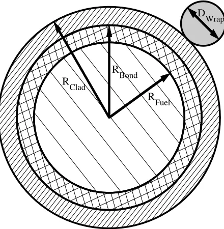
Note the individual rods in Fig. 1.2 are cylindrical and are arranged into a hexagonal assembly. The
basic geometry is a metallic fuel material within stainless steel cladding. The gap between the fuel and cladding is filled by sodium bond to improve thermal conductivity across the gap. The rod is helically
wrapped by a steel wire to ensure separation between rods that will allow for coolant flow. The wire wrap
also serves to encourage the mixture of coolant within the assembly. (Note: wire wrap is omitted from Fig. 1.2.) Many rods are then assembled into an assembly and surrounded by a hexagonal can made of
steel. This can aids in structural stability and prohibits cross-flow of coolant between assemblies.
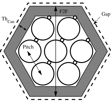
The dimensions within a single rod are shown in Fig. 1.3 and the dimensions within a hexagonal assembly can are shown in Fig. 1.4. In Fig. 1.4,Thcan is the thickness of the assembly can,F2Fis the
Figure 1.1Example of Fast Reactor Materials based on MONJU.
R
Fuel
R
Bond
R
Clad
D
Wrap
Figure 1.3Dimensions of Thermal Hydraulic Rod Model (not to scale).
pitch.AP >F2Fto account for inter-assembly sodium gaps (see “Gap” in Fig. 1.4).
Atot al =
√
3 2 AP
2 (1.1)
Abox =
√
3 2
F2F2− (F2F−2T hcan)2
(1.2)
Awr ap = Nr odπ 4D
2
wr ap (1.3)
Aclad= Nr odπ(RC2 −RB2) (1.4)
Abond= Nr odπ(R2B−R2F) (1.5)
Af uel = Nr odπRF2 (1.6)
Acool= Atot al−Abox− Awr ap− Aclad−Abond−Af uel (1.7)
Astr uct = Abox+ Awr ap+ Aclad (1.8)
Calculating the areas as above allows for calculation of cross-sectional area fractions. Assuming constant dimensions in the axial direction, these area fractions are equivalent to volume fractions and are useful
for neutron cross section homogenization. Additionally, these formulae allow for thermal expansion as
ThCan
F2F
Pitch
Gap
Figure 1.4Dimensions of Hexagonal Can (not to scale).
1.3
Cross Section Treatment
Reactor materials are “smeared” into homogeneous regions. This treatment is common to fast reactors because of the relatively large neutron mean-free-paths compared to the scale of material dimensions.
Additionally, the neutron distribution will be modeled using the neutron diffusion equation which cannot
accurately resolve small geometric details. The natural choice for these homogeneous regions are the hexagonal assemblies themselves. Materials are permitted to be heterogeneous axially. For this work,
four distinct regions are modeled within a hexagonal assembly: fuel, bond, coolant, and steel. Steel
material includes cladding, wire wrap, and assembly can. These four regions are then homogenized into a hexagonal assembly.
For simplified analytic and benchmark problems, cross sections are specified by the problem. For
realistic simulations, multigroup microscopic cross sections are generated using the computer program MC**2 [Lee12]. The cross section generator uses 2,082 fine energy groups to collapse down to an arbitrary
number of coarse energy groups. For this simulation, the recommended and default 33-group energy
structure is used. However, the methods in this work are implemented generally and are not dependent on a particular energy group structure. MC**2 solves the infinite-homogeneous (zero-dimension) neutron
transport equation for isotopic number densities as input by the user. Cross sections for each assembly
type are generated separately to accurately simulate the neutron energy spectrum within the assembly. This procedure results in a unique material cross sections for each assembly type. For example, each
assembly type contains steel; therefore, there will be a separate steel cross section for each assembly type
Table 1.1Temperatures Selected for Cross Section Libraries.
Library Tcool[K] Tclad[K] Tf uel[K]
1 628.15 628.15 628.15
2 708.65 757.50 807.15
3 896.87 920.47 961.46
4 1072.81 1114.83 1183.14
the media’s fission spectrum. Non-fissile homogenized mixtures, such as control assemblies or reflector
assemblies, the default238U fission spectrum is assumed.
Cross section libraries are generated for several different temperatures to capture
temperature-dependent cross section effects. These libraries are then used during the simulation to calculate cross
sections as a function of material temperatures. The fuel, clad, and coolant temperatures in a simulated reactor can be calculated with a thermal hydraulic model (see Chapter 4). However, the temperatures
calculated in the thermal hydraulic model are functions of reactor power and coolant mass flow rate. These
parameters are not known before the simulation for a general reactor. Instead, a simplified one-dimensional, single-channel model is used to estimate temperatures for cross section library generation. This model is
based on the axial convection and radial conduction models in Chapter 4. The simulation model can use
general cross section library temperatures and a general number of temperature libraries. A user may select the number of cross section libraries and specify the temperatures for which the libraries apply in
a general manner. Typical cross section library temperatures for simulating liquid metal cooled, metal
fueled, fast reactors are given in Table 1.1.
Note that the maximum temperatures in Table 1.1 are greater than temperatures observed at typical
reactor operating conditions. This is necessary so that even at perturbed reactor conditions (e.g. 110%
full power), the peak core temperatures can still be interpolated within the libraries.
Cross sections are homogenized within each hexagonal assembly using isotopic microscopic cross
sections from MC**2 and user input number densities. Homogenization is performed in two steps: first, isotopic homogenization and second, volumetric homogenization. Isotopic homogenization is performed
by summing microscopic cross sections and associated number densities. Let σi,j,x,g represent the
microscopic cross section for isotopei, in region j, for reaction typex, and energy groupgas output by MC**2.σi,j,x,ghas units of area. Then, letNi,jrepresent the atom number density for isotopeiin region
jas input by the user.Ni,jhas units of inverse volume. The macroscopic cross section can then be defined
Σj,x,g=
Ni s o Õ
i=1
whereΣj,x,gis the macroscopic cross section in region j, for reaction type x, and energy group g. In Eq. (1.9),Nisorepresents the number of isotopes in region j. Note thatΣj,x,gwill have units of inverse length.
Next, volumetric cross section homogenization is performed using volume fractions. Assuming
dimensions do not change axially within a hexagonal assembly, the areas calculated in Eq. (1.1) through Eq. (1.8) can be used to calculate area fractions. These area fractions can subsequently be treated as
volume fractions. Using the definition of macroscopic cross sections from Eq. (1.9), the volumetrically
homogenized macroscopic cross section is
Σx,g=
ÍNr e g
j=1 Σj,x,gVj ÍNr e g
j=1 Vj
(1.10)
whereVjis the volume or area occupied by regionjin the hexagonal assembly andNr egis the number of
regions in the hexagonal assembly. Typically,Nr eg =4 with unique regions for fuel, sodium bond, sodium coolant, and steel structural material. After homogenizing cross sections isotopically and volumetrically,
the diffusion coefficient for energy groupg,Dg, can be calculated as
Dg = 1
3Σtr,g (1.11)
where Σtr,g represents the macroscopic transport cross section for energy group g. Σtr,g has been homogenized according to Eq. (1.9) and Eq. (1.10). Note thatDgwill have units of length.
1.4
Thesis Organization
In Chapter 2, the derivation of the FEM solution to the multigroup neutron diffusion equation is presented. Special attention is paid to triangular and wedge elements. The resulting eigenvalue problem is solved
using the Power Method. Results from the diffusion solution are verified in two-dimensional and
three-dimensional problems with both analytic and benchmark solutions. These verification problems for the neutron diffusion equation are presented in Chapter 3.
Chapter 4 presents the formulation of axial heat convection and radial heat conduction models for a
typical fast reactor. These models are used to calculate material temperatures and update cross sections for the simulation. Results of the numerical model are compared to analytical models and example material
temperatures are shown.
In Chapter 5 a simplified thermal expansion model is presented. The model assumes linear thermal expansion for given material properties and user-specified thermal expansion temperatures. A simple
The combination of all of these models allows for the realistic simulation of a fast reactor. In Chapter 6,
the multiphysics models are coupled and investigated for a benchmark reactor problem. Using this
benchmark reactor and the models described, multiphysics reactivity feedback coefficients are estimated. Finally, Chapter 7 presents a summary and the conclusions of this research. Additionally,
CHAPTER
2
FINITE ELEMENT NEUTRON
DIFFUSION
2.1
Introduction
This chapter will describe the solution of the multigroup neutron diffusion equations for general
geometry via the Finite Element Method (FEM). The solution method and derivations here are general
to the multigroup neutron diffusion equation and its application to any standard reactor geometry is straightforward. For typical fast reactor applications, diffusion theory approximates the neutron distribution
within the reactor well. The diffusion approximation is a standard assumption for fast reactors because
neutron mean-free-paths within the reactor are large relative to material dimensions.
Spatial discretization will be done with the FEM. This spatial discretization method is selected for
several reasons. It allows for easily increasing the spatial convergence order of the method by increasing the order of the elements without refining the mesh. For example, with a given mesh, quadratic elements
instead of linear elements could be used to spatially refine the solution. Additionally, coordinates of
nodes and elements can be easily updated to reflect physical phenomena, such as thermal expansion (see Chapter 5). Finally, material properties are calculated on an element basis allowing for detailed updates to
2.2
Multigroup Neutron Diffusion Equation
In the multigroup neutron diffusion equation, an energy structure is described by the set of energies{Eg}
forg=1,2, . . . ,G. By convention, the energy groups are arranged in order of decreasing energy.
0< EG <EG−1 < . . . <E2 < E1 (2.1)
Multigroup neutron cross sections can be calculated using this energy group structure from energy
dependent cross sections, and a representative flux spectrum. Generation of multigroup neutron cross
sections is performed using MC**2 and is described in §1.3.
In conventional notation, the multigroup neutron diffusion equation can be written as
− ∇ · (Dg(r)∇φg(r))+Σt,g(r)φg(r)= f
χg(r)
keff G
Õ
g0=1
νΣf,g0(r)φg0(r)+
G
Õ
g0=1
Σs,g0→g(r)φg0(r) (2.2)
where
r =spatial position vector,
Dg(r) =diffusion coefficient for energy groupg[cm],
φg(r) =scalar neutron flux for energy groupg
h 1 cm2s
i ,
Σt,g(r) =macroscopic total cross section for energy groupg cm1 , fχg(r) =effective fission spectrum for energy groupg,
keff =effective neutron multiplication factor,
νΣf,g(r) =number of fission neutrons times macroscopic fission cross section in energy groupg cm1 ,
Σs,g0→g(r)=macroscopic scatter cross section from energy groupg0to energy groupg 1 cm
,
G =total number of energy groups.
The total neutron cross section includes the contribution due to within-group scattering; that is, due
toΣs,g→g. This can be subtracted from both sides of Eq. (2.2) for simplicity and numeric efficiency. Rewriting Eq. (2.2) with this modification yields
− ∇ · (Dg(r)∇φg(r))+Σr,g(r)φg(r)= f
χg(r)
keff G
Õ
g0=1
νΣf,g0(r)φg0(r)+
G
Õ
g0=1
g0 ,g
Σs,g0→g(r)φg0(r) (2.3)
For simplicity, the neutron sources in Eq. (2.3) can be combined into a single term as
− ∇ · (Dg(r)∇φg(r))+Σr,g(r)φg(r)=qg(r) (2.4) whereqg(r)is the combined neutron source at positionrfor energy groupgand is expressed as
qg(r)=qf iss,g(r)+qu p,g(r)+qdown,g(r) (2.5)
with contributing terms
qf iss,g(r)= fχg
(r)
keff G
Õ
g0=1
νΣf,g0(r)φg0(r), (2.6)
qu p,g(r)=
G
Õ
g0=g+1
Σs,g0→g(r)φg0(r), (2.7)
qdown,g(r)=
g−1 Õ
g0=1
Σs,g0→g(r)φg0(r), (2.8)
where the difference betweenqu pandqdown are the limits of the summation.qu prepresents the neutron source due to scattering from lower energy groups (up-scattering) andqdown represents the neutron
source due to scattering from higher energy groups (down-scattering). This form allows for operator
splitting of the neutron source term. In an iterative scheme, it will be necessary for fission and up-scatter sources to use a different flux iterate than down-scatter so this separation of sources will prove useful (see
§2.4.2).
The combined source form is useful for solving the multigroup neutron diffusion problem for an arbitrary number of groups. Eq. (2.4) is solved for each energy group and interaction between groups is
described in the source term,qg(r). In other literature, the multigroup equation may be solved for all groups
simultaneously by treating interaction between groups explicitly. By solving each group independently (as done here) the method remains general. Additionally, for many-group energy structures, as common to
fast reactor applications, solving each group independently is typically more computationally efficient as
such linear systems have favorable conditioning and are dimensionally smaller. Finally, fast reactors are also dominated by down-scatter as opposed to thermal reactors which experience significant up-scatter at
thermal energies. This fact implies that the termqu p,g(r)will not have to be updated frequently in fast
reactor simulations and the one group at-a-time solution method will benefit.
Typically, reactor materials are described isotopically and χmay be specified isotopically. However,
isotopic description,qf iss,g(r)is given as
qf iss,g(r)= Ni s o
Õ
i=1
χi,g(r)©
«
G
Õ
g0=1
νΣf,i,g0(r)φg0(r)ª
®
¬
(2.9)
where χi,g(r)is the isotopic fission spectrum and Niso is the number of isotopes at positionr. Next, requireqf iss,g(r)to have the form of Eq. (2.10).
qf iss,g(r)= fχg(r)
Ni s o Õ
i=1
G
Õ
g0=1
νΣf,i,g0(r)φg0(r) (2.10)
Setting Eq. (2.9) equal to Eq. (2.10) yields the expression forfχg(r)based on isotopic data.
fχg(r)= ÍNi s o
i=1 χi,g(r)
ÍG
g0=1νΣf,i,g0(r)φg0(r)
ÍNi s o
i=1 ÍG
g0=1νΣf,i,g0(r)φg0(r)
(2.11)
Note that Eq. (2.11) requires the solutionφg(r). Ultimately, the flux is unknown but will be solved in an iterative manner. Eq. (2.11) implies thatfχg(r)must be updated for each iteration of the solution (see Step
9 in Algorithm 2.2).
2.3
Formulation of Finite Element Equations
This section presents the derivation of the spatial discretization of the multigroup neutron diffusion
equation based on the FEM. The method results in a linear system of equations for a fixed source iteration. Details are also provided on constructing the finite element matrix for use with triangular and wedge
elements.
2.3.1 Derivation
The remaining continuous variable in the problem to be discretized in Eq. (2.4) is the spatial variabler. This will be discretized according to the FEM. The problem is solved in a finite domainr∈Ωwhere∂Ω
represents the boundary of the domain and some boundary condition is specified. Boundary condition
options include:
1. Mirror.∇φg(r) ·nˆ =0 forr∈∂Ω.
2. Albedo.Dg(r)∇φg(r) ·nˆ +αφg(r)=0 forr∈∂Ω, whereα∈Ris a scalar constant specified by the user. For non-reentrant boundary condition,α= 12.
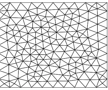
Figure 2.1Example of Rectangular Unstructured Mesh.
ˆ
n represents the unit outward normal vector at the boundary ∂Ω. (Note: the order of the above list corresponds to the order of boundary condition precedent in code with the greater the integer, the greater
the precedent.)
Begin by partitioning the spatial domainΩinto a set of finite elements.
Ω=Ω1∪Ω2∪Ω3∪. . .∪ΩNE (2.12)
such thatΩ= {Ωe}fore=1,2, . . . ,NE is a set of non-overlapping elements
Ωi∩Ωj =∅, fori, j, (2.13)
andNE is the total number of elements. Elements are in an unstructured mesh and can be generated by any number of mesh generation methods (e.g. Delaunay triangulation) to describe the geometry of the
problem. An example of an unstructured mesh generated for a rectangular domain is shown in Fig. 2.1.
Proceeding with the Galerkin FEM, Eq. (2.4) is multiplied by a testing functionv(r) ∈H1(Ω)where
His the Sobolev space.
− ∇ · (Dg(r)∇φg(r))v(r)+Σr,g(r)φg(r)v(r)=qg(r)v(r) (2.14) Then, Eq. (2.14) is integrated over the problem domain. This integration yields the Weak Form or Variational Form of the problem.
− ∫
Ω
∇ · (Dg(r)∇φg(r))v(r) dr+
∫
Ω
Σr,g(r)φg(r)v(r) dr= ∫
Ω
qg(r)v(r) dr (2.15)
For the purposes of this work, material cross sections and the neutron source,qg,e, are assumed to
each element. To calculate a constant neutron source within an element, Eq. (2.5) is used to calculate the
average neutron source,qg,e, in an element.
qg,e =qf iss,g,e+qu p,g,e+qdown,g,e (2.16)
g
χg,e =
ÍNi s o
i=1 χi,g,e
ÍG
g0=1νΣf,i,g0,eφg0,e
ÍG
g0=1Íi=1Ni s oνΣf,i,g0,eφg0,e
(2.17)
qf iss,g,e = χgg,e keff
G
Õ
g0=1
νΣf,g0,eφg0,e (2.18)
qu p,g,e = G
Õ
g0=g+1
Σs,g0→g,eφg0,e (2.19)
qdown,g,e = g−1 Õ
g0=1
Σs,g0→g,eφg0,e (2.20)
Note that in Eq. (2.17), χgg,e must now be calculated for each finite element. For first-order, linear
implementations of the FEM, the element-average fluxφg,eis
φg,e = 1
Np Np Õ
i∈Ωe
φi,g (2.21)
whereNpis the number of nodes on the element andi ∈Ωe is the summation over all nodes in element
Ωe. For example, a triangle hasNp =3 and a wedge hasNp =6.
Given constant material properties and constant neutron source over the element, the integrals in
Eq. (2.15) can be partitioned into a sum of integrals over the elements in the domain assuming the non-overlapping set of elements from Eq. (2.12) and Eq. (2.13).
−
NE Õ
e=1
Dg,e
∫
Ωe
∇ · ∇φg(r)v(r) dr+ NE Õ
e=1
Σr,g,e
∫
Ωe
φg(r)v(r)dr=
NE Õ
e=1
qg,e
∫
Ωe
v(r) dr (2.22)
The Second Green’s Theorem is used to rewrite the integral in the first term. A proof invoking the Second
Green’s Theorem has been published by Li et al. [Li18]. The Second Green’s Theorem is
− ∫
Ωe
∇ · ∇φg(r)v(r) dr=− ∫
∂Ωe
(∇φg(r) ·n)ˆ v(r)ds+
∫
Ωe
∇φg(r) · ∇v(r)dr (2.23)
where ∇φg(r) ·nˆ is the outward normal derivative and the integral∫∂Ω· ds is a line integral in two dimensions or a surface integral in three dimensions. Recognizing that this quantity will only be relevant
condition. Specifically, the albedo boundary condition which has the form
Dg(r)∇φg(r) ·nˆ +αφg(r)=0 (2.24)
Dg(r)∇φg(r) ·nˆ =−αφg(r) (2.25)
forr∈∂Ω. Note that all allowed boundary conditions (mirror, albedo, and zero-flux) can be specified as an albedo condition. For mirror boundaries,α=0 and for zero-flux boundaries,α→ ∞. Substituting
Eq. (2.23) into Eq. (2.22).
−
NE Õ
e=1
Dg,e
∫
∂Ωe
v(r)∇φg(r) ·nˆ ds+ NE Õ
e=1
Dg,e
∫
Ωe
∇φg(r) · ∇v(r) dr+
NE Õ
e=1
Σr,g,e
∫
Ωe
φg(r)v(r) dr=
NE Õ
e=1
qg,e
∫
Ωe
v(r)dr (2.26)
Assuming the outward normal derivative is specified in the form of an albedo boundary condition withα
constant throughout the problem boundary as in Eq. (2.25).
NE Õ
e=1
α
∫
∂Ωe
v(r)φg(r)ds+ NE Õ
e=1
Dg,e
∫
Ωe
∇φg(r) · ∇v(r) dr+
NE Õ
e=1
Σr,g,e
∫
Ωe
φg(r)v(r) dr=
NE Õ
e=1
qg,e
∫
Ωe
v(r)dr (2.27)
Next, for the Galerkin formulation of the FEM, the function of interestφg(r)is assumed to be a linear
combination of chosen basis functions,Ni, as
φg(r)=
DOF
Õ
i=1
υi,gNi(r) (2.28)
where coefficientsug ={υi,g}are unknown and will be determined andDOFis the total number degrees of freedom of the problem. TypicallyDOFis the number of nodes less any nodes for which the flux is
fixed (e.g. zero-flux nodes).
Typically, basis functions have unit magnitude and are centered at the node points so the coefficients
υi,gare the FEM solution at the nodes. It is also convenient for basis functions to have compact support. That is, basis functions are created such that they are zero almost everywhere except some minimal region.
Compact support in this implementation is chosen such that basis functions have unit value on a single mesh node and are zero on all other mesh nodes. Basis functions are typically piecewise continuous
§2.3.2. Linear and quadratic polynomials are common; but, for the work presented here, only linear basis
functions are explored.
The test function,v(r) ∈H1(Ω), is also chosen as a linear combination of the same basis functions. v(r)=
DOF
Õ
j=1
Nj(r) (2.29)
The magnitude of the testing function is arbitrary so the magnitude is set to unity. Eq. (2.28) and Eq. (2.29) are inserted into Eq. (2.27).
NE Õ
e=1
α
DOF
Õ
i=1
υi,g
∫
∂Ωe
Ni(r)Nj(r)ds+ NE Õ
e=1
Dg,e DOF
Õ
i=1
υi,g
∫
Ωe
∇Ni(r) · ∇Ni(r) dr+
NE Õ
e=1
Σr,g,e
DOF
Õ
i=1
υi,g
∫
Ωe
Ni(r)Nj(r)dr=
NE Õ
e=1
qg,e DOF
Õ
i=1 ∫
Ωe
Ni(r)dr (2.30)
Eq. (2.30) can be rearranged as a linear system of equations.
DOF
Õ
i=1
υi,g DOF
Õ
j=1
NE Õ
e=1
α∫
∂Ωe
Ni(r)Nj(r)ds+ NE Õ
e=1
Dg,e
∫
Ωe
∇Ni(r) · ∇Nj(r)dr+
NE Õ
e=1
Σr,g,e
∫
Ωe
Ni(r)Nj(r) dr
!
=
DOF
Õ
i=1
NE Õ
e=1
qg,e
∫
Ωe
Ni(r)dr
!
(2.31)
Which can be written in the notation common to the mathematical discussions of the FEM
ag(Ni,Nj)= fg(Ni) (2.32)
whereag(Ni,Nj)is the bilinear form of the FEM for groupgand fg(Ni)is the linear form of the FEM for groupg. Eq. (2.31) can also be written in matrix format as
Agug=fg (2.33)
whereug={υi,g}.
The diffusion coefficient Dg(r)is non-zero and bounded and the removal cross sectionΣr,g(r)is bounded. Given these conditions, the Lax-Milgram Lemma implies the solution to the FEM equations as
derived here is both unique and bounded [Li18]. This is not the entire solution description as the source
functionqg(r)is updated on each power iteration (see §2.4). What the satisfaction of the Lax-Milgram Lemma does imply is, for a fixed source problem in a given power iteration, a unique and bounded
In the matrix notation of Eq. (2.33), matrixAgis described by integral quantities, vectorugis the unknown magnitudes of the basis functions{υi,g}, and vectorfgis described by source integral quantities. Inspecting the finite elements matrixAgand the vectorfgfor elementereveals
Ai,j,g,e =α
∫
∂Ωe
Ni(r)Nj(r) ds+Dg,e
∫
Ωe
∇Ni(r) · ∇Nj(r)dΩe+Σr,g,e
∫
Ωe
Ni(r)Nj(r)dΩe, (2.34) fi,g,e =qg,e
∫
Ωe
Ni(r)dΩe. (2.35)
Then, all element data can be combined as
Ai,j,g = NE Õ
e=1
Ai,j,g,e, (2.36)
fi,g = NE Õ
e=1
fi,g,e, (2.37)
which leads to the natural population of the matrixAgin an element-by-element procedure. MatrixAgis assembled by looping through all elements and summing their contribution to the matrix. Note that the contribution due to the surface integral will be zero in elements not on the problem boundary and may
also be zero for problems with select boundary conditions. See §2.5.3 for boundary condition discussion.
The population of the vectorfgis done similarly in an element-by-element fashion. Then, the matrixAg and the vectorfgare known for each energy group. The equations are solved for one energy group at a time andφgis calculated and stored.
The above derivation reduces to a linear system of equations. These equations are constructed from the integral quantities specified by the FEM and the coefficients given by the cross sections. The integral
quantities themselves are expressed explicitly in the §2.3.2.
2.3.2 Matrix Quantities
For selected simple elements, the integral quantities described in Eq. (2.34) and Eq. (2.35) have exact analytic forms. For this work, linear triangles and linear wedges are investigated and many of the
integrals have exact expressions. If these quantities cannot be expressed exactly, or doing so would be
computationally inefficient, numerical quadratures are used. Given proper selection of the quadrature set, a quadrature rule can express the integrals exactly. This will be discussed in §2.3.3.
2.3.2.1 Linear Triangles
Linear triangles are common to two-dimensional FEMs and have been investigated in many methods for
(a)General Triangle Element.
0 0.2 0.4 0.6 0.8 1 0
0.2 0.4 0.6 0.8 1
(b)Reference Triangle.
Figure 2.2Description of Triangle Elements.
It is difficult to analytically calculate the desired integral quantities for an arbitrary triangle. Instead, a
simplified reference element is created and quantities are calculated for the reference element and then translated to the arbitrary element using a Jacobian. The reference triangleTr e f is located inξ ∈ [0,1]and
η∈ [0,1−ξ]. General and reference triangles are shown in Fig. 2.2. The basis functions are zero outside of the reference triangle. Within the reference triangle, basis functions for the triangle are provided in the natural coordinates ofTr e f.
Ni(ξ, η)=0 ∀(ξ, η)<Tr e f (2.38)
N1(ξ, η)=ξ (2.39)
N2(ξ, η)=η (2.40)
N3(ξ, η)=1−ξ−η (2.41)
For linear triangles, simple expressions for the integral quantities for an arbitrary triangle can be
For a general triangle with corners(xi,yi)withi=1,2,3
∫
Ωe
∇Ni(r) · ∇Nj(r)dr= 1 4Ae
((xi+1−xi+2)(xj+1−xj+2)+(yi+1−yi+2)(yj+1−yj+2)), (2.42)
∫
Ωe
Ni(r)Nj(r)dr= Ae
12(1+δi j), (2.43)
∫
Ωe
Ni(r)dr= Ae
3 , (2.44)
∫
∂Ωe
Ni(r)Nj(r)ds= Le
6 (1+δi j), (2.45)
where Ae is the area of the triangular element,Leis the length of the edge between nodeiand nodej,
andδi j is the Kronecker delta. The Kronecker delta is defined as
δi j =
0 ifi, j,
1 ifi= j.
(2.46)
The area of a triangle in three dimensions is calculated for a triangle with corner coordinatesci =(xi,yi,zi) withi=1,2,3. That is,ciis the coordinates of corneri. Calculation of the area of a general triangle is then given by the vector operations
a=c2−c1, (2.47)
b=c3−c1, (2.48)
Ae = 1
2|a×c|, (2.49)
Ae = 1 2
p
(a2b3−a3b2)2+(a3b1−a1b3)2+(a1b2−a2b1)2, (2.50)
where ai is theith component of vectoraand bi is theith component of vectorb. For higher order triangular elements (e.g. quadratic or cubic elements), it may be necessary to employ a quadrature to
calculate the necessary integral quantities.
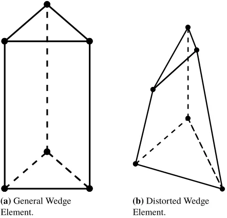
2.3.2.2 Linear Wedges
A wedge element is a pentahedron with six corner nodes, and is sometimes referred to as a triangular
prism. A simple example of a wedge is an extruded triangle. However, unlike an extruded triangle, the
exact geometric relation of corner nodes in a wedge is not fixed and the nodes are free to expand and distort. An example of typical and distorted wedge elements are shown in Fig. 2.3. These elements are
(a)General Wedge Element.
(b)Distorted Wedge
Element.
Figure 2.3Description of Wedge Elements.
Fast reactors typically have hexagonal-z geometry so wedge elements are a natural choice for this
coordinate system. Reactor geometries are also typically described in lattices so the wedge element allows
for easily “stacking” lattices on top of each other.
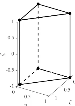
The reference wedgeWr e f is located inξ ∈ [0,1],η ∈ [0,1−ξ], andζ ∈ [−1,1]. The coordinate
system of the reference wedge is shown in Fig. 2.4. The basis functions are zero outside of the reference
wedge and are provided within the reference wedge.
Ni(ξ, η, ζ)=0 ∀(ξ, η, ζ)<Wr e f (2.51)
N1(ξ, η, ζ)=
1
2(1−ζ)(1−ξ−η) (2.52)
N2(ξ, η, ζ)= 1
2(1−ζ)ξ (2.53)
N3(ξ, η, ζ)=
1
2(1−ζ)η (2.54)
N4(ξ, η, ζ)=
1
2(1+ζ)(1−ξ−η) (2.55)
N5(ξ, η, ζ)= 1
2(1+ζ)ξ (2.56)
N6(ξ, η, ζ)=
1
2(1+ζ)η (2.57)
The integrals of the basis function over the element are given in Eq. (2.58) through Eq. (2.60). The
0 -1 0.5 0 -0.5 0.5 1 0 1 0.5 1
Figure 2.4Description of Reference Wedge.
wedge, the integral quantities are
∫
Ωe
Ni(r)Nj(r)dr= Ve
144 © «
4 2 2 2 1 1
2 4 2 1 2 1
2 2 4 1 1 2
2 1 1 4 2 2
1 2 1 2 4 2
1 1 2 2 2 4
ª ® ® ® ® ® ® ® ® ® ® ¬ , (2.58) ∫ Ωe
Ni(r)dr= Ve
12, (2.59)
∫
∂Ωe
Ni(r)Nj(r)ds=
A4
12(1+δi j) if triangular surface,
A
36(1+δi j)(1− 1
2δi,(5−j)) if quadrilateral surface,
(2.60)
whereVeis the volume of the element,A4is the area of the triangular surface, andAis the area of the
quadrilateral surface. The matrix in Eq. (2.58) is indexedMi jwherei,j=1,2, . . . ,6. The indices,i j, are the indices of the six basis functions corresponding toNi(r)andNj(r)respectively.
Notice the integral containing the gradient operator has been omitted because it is computed using a
quadrature. If it could be computed analytically, it would be less computationally efficient than using a
quadrature.
A4is computed according to Eq. (2.50) andAis computed as the sum of the area of two triangles,
employing the same formula. For a simple extruded triangle, the volume calculation is straightforward
to each other makes the volume of the element difficult to calculate. Therefore, the Jacobian is used to
calculateVe. For more detail, see §2.3.3, especially Table 2.2.
2.3.3 Quadratures
Quadratures are sets of coordinates and weights which are used to approximate an integral. For a given
set of weights,{wi}, and a set of coordinates,{xi}, an integral can be represented as the sum
∫
Ω
f(x) dΩ≈
N
Õ
i=1
f(xi)wi (2.61)
whereΩ is an arbitrary domain described by{xi}. A quadrature, such as the one in Eq. (2.61), can be designed to exactly integrate a polynomial of ordern. It is not necessarily true that the number of
quadrature points,N, will equal the order of the polynomial exactly integrated,n. Generally,n, N. For one-dimensional integrals, the Gaussian quadrature is common and the most compact quadrature.
The Gaussian quadrature exactly integrates a polynomial of ordernusing exactlyN =npoints. For the
one-dimensional Gaussian quadrature, the number of points in the quadrature is the same as the order of the quadrature andn=N.
Two-dimensional and three-dimensional quadratures are necessary for the FEM. Triangular quadratures
are not as simple to derive as line quadratures and the number of points need not equal the order of the polynomial integrated. The triangular quadrature as implemented here is symmetric and open. That is,
there are no points on the boundary of the triangle [Dun85]. Any triangular quadrature will suffice that exactly integrates polynomials of a given order. There is no fixed relationship betweennandN and for
this quadrature,n,N.
Quadrilateral quadrature sets are simply tensor products of two line Gaussian quadratures. For an ordernpolynomial, nowN2=npoints are required.
Wedge quadrature sets are simply tensor products of a line Gaussian quadrature and a triangular
quadrature. Again, there is no fixed relationship betweennandN.
Though only linear functions are used here, basis functions are generally polynomials of first, second,
or third order; that is, linear, quadratic, or cubic functions. The quadratures described are capable of
exactly integrating polynomial functions of given order so there exists a quadrature order that will exactly integrate the finite element quantities to numeric precision. The table of the order required for exact
integration are provided in Table 2.1.
All of the quadratures described here are tabulated for a reference element be it a line, triangle, quadrilateral, or wedge. Integration in the FEM is performed on an arbitrary element in space. Therefore, it
Table 2.1Quadrature Orders for FEM Quantities.
Quantity Linear Quadratic Cubic
∫
ΩNi(r) dΩ 1 2 4
†
∫
ΩNi(r)Nj(r)dΩ 2 4 6
∫
Ω∇Ni(r) · ∇Nj(r)dΩ 2 3 5
†A third-order quadrature would be exact but the triangular quadrature would
have negative weights so a fourth order quadrature is selected.
Table 2.2Jacobi for Selected Elements.
Element J
Triangle Ae Quadrilateral 14Ae Wedge 12Ve
coordinates from domainΩto the reference domainΩr e f can be written ∫
Ω
f(x)dΩ=
∫
Ωr e f
f(x)|J| dΩr e f ≈
N
Õ
i=1
wif(xi)|Ji| (2.62)
whereJis the Jacobian matrix,Jiis the Jacobian matrix at quadrature coordinatexi, and|·|represents the matrix determinant. Notationally,J = |J|and is termed the Jacobi.
Isoparametric elements are elements in which shape functions can be used to relate global coordinates,
(x,y,z), to local coordinates(ξ, ζ, η). Generally, non-curved elements are isoparametric. For isoparametric elements, such as triangles and wedges, the Jacobi is constant over the element and can be pre-calculated. Pre-calculating the Jacobi avoids populating and evaluating the determinant of a matrix for each integration
point. For the elements of concern, these values are presented in Table 2.2 [Fel04].
For the general element, the Jacobian matrix,Ji, is calculated at each point of the quadrature(ξi, ζi, ηi) as described in Eq. (2.63).
Ji =
© « ÍNP
k=1
∂Nk
∂ξ
(ξi,ζi,ηi)
xk ÍkN=P1 ∂N∂ζk
(ξi,ζi,ηi)
xk ÍkN=P1 ∂N∂ηk
(ξi,ζi,ηi)
xk
ÍNP
k=1
∂Nk
∂ξ
(ξi,ζi,ηi)
yk ÍkN=P1 ∂N∂ζk
(ξi,ζi,ηi)
yk ÍkN=P1 ∂N∂ηk
(ξi,ζi,ηi) yk
ÍNP
k=1
∂Nk
∂ξ
(ξi,ζi,ηi)
zk ÍNk=P1 ∂N∂ζk
(ξi,ζi,ηi)
zk ÍkN=P1 ∂N∂ηk
(ξi,ζi,ηi)
In Eq. (2.63),NP is the number of points in the element,Nk(r)is the basis function centered at thekth
corner, and for corner coordinates(xk,yk,zk)fork =1,2, . . . ,NP.
With the Jacobian populated as Eq. (2.63),J= |J|is simply the matrix determinant. For the quadrature integration of derivative quantities as necessary in the FEM, the derivatives must also be translated from
the reference element to the spatial element. This is performed according to Algorithm 2.1. The notation is dense as the method requires two sets of coordinates. First, the coordinate in the reference element
(ξ, ζ, η)and second, the coordinate in Cartesian space(x,y,z).
The vectordi,(ξ,ζ,η)is the gradient vector forNiwith respect to the reference coordinates(ξ, ζ, η).
di(ξ,ζ,η)=∇(ξ,ζ,η)Ni(r) (2.64)
Vectordi,(x,y,z)is the gradient vector forNi with respect to the Cartesian coordinates(x,y,z).
di,(x,y,z)=∇(x,y,z)Ni(r) (2.65)
In Algorithm 2.1, the quadrature has points{xp}and weights{wp}forp=1,2, . . . ,Nand the value of the integral,v, is represented by Eq. (2.66).
v=
∫
Ωe
∇(x,y,z)Ni(r) · ∇(x,y,z)Nj(r) dΩe (2.66)
Algorithm 2.1Integral of Derivative with Jacobian Method.
1: v=0
2: forp=1,NPdo
3: Calculate the JacobianJas in Eq. (2.63).
4: Calculate the vectordi,(ξ,ζ,η)at quadrature pointxp.
5: Calculate the vectordj,(ξ,ζ,η)at quadrature pointxp.
6: Invert and store the JacobianJ−1.
7: Calculate the vectordi,(x,y,z)=di,(ξ,ζ,η)J−1.
8: Calculate the vectordj,(x,y,z)=dj,(ξ,ζ,η)J−1.
9: v =v+di,T(x,y,z)dj,(x,y,z)
wp|J|
2.4
Power Iterations
The FEM is used to solve a fixed source problem for a given source distribution qg(r). However, for
known. For eigenvalue problems, the problem does not have a fixed source and the system has many
solutions. The method of Power Iterations allows eigenvalue problems to be solved iteratively for the
fundamental eigenvalue and eigenvector.
2.4.1 Convergence of Power Iteration Method
Noting the FEM equations can be written as matrix form Eq. (2.33), the discretized multigroup neutron
diffusion equation can be rewritten as
B(Φ,keff)Φ= 1
keffMΦ (2.67)
whereΦis the vector of the flux containing all energy groups, matrixBcontains the diffusion, removal, and all scattering terms, andMincludes all fission generation and operates onΦandkeff.Bis an S-matrix and its inverse,B−1, exists and has all positive elements [Nak77]. Therefore, Eq. (2.67) can be rewritten as
Φ= 1
keffRΦ (2.68)
where
R=B−1M. (2.69)
MatrixMis non-symmetric and is non-negative andBis an S-matrix; therefore,Ris a non-symmetric, non-negative matrix.
In the solution of Eq. (2.2), the largest eigenvalue,keff, is desired along with its associated eigenvalue,
φg. The solution can be found using the method of power iterations which can be written as
Φ(s+1) = 1
keff(s)
RΦ(s), (2.70)
keff(s+1) =keff(s)hw,Φ
(s+1)i
hw,Φ(s)i , s =1,2, . . . ,∞, (2.71)
wheresis the iteration counter,wis a weighting vector andhw,Φiis an inner-product. According to the Perron-Frobenius theorem, a matrix with the properties ofRhas a unique, positive eigenvalue, greater in magnitude than the modulus of all other eigenvalues of the matrix [Geh92; Nak77]. The weighting vector
wis arbitrary but does affect convergence rate. For this work,w= {νΣf}such that the inner product
h{νΣf},Φirepresents the summation of the fission neutron production rate throughout all energy groups and all elements.
It can then be shown in that the method of power iterations described in Eq. (2.70) and Eq. (2.71)
enumeration, allow the eigenvalue to be rewritten as
µ= 1
keff
. (2.72)
The eigenvectorsunand corresponding eigenvalues,µn, ofRare defined by
un= µnR un. (2.73)
It may be proved that all eigenvalues,µ, are real, positive, and distinct. The eigenvalues are then numbered
in the sequence
µ0< µ1< µ2 <· · · < µN (2.74)
whereNis the rank of the problem. The eigenvectors have the orthogonality relations
uTnum=0 forn,m (2.75)
whereuTuis the vector inner-product. Assume eigenvectors are normalized such that
uTnun=1 forn=1,2, . . . ,N. (2.76)
The initial vector,Φ(0), may be expressed as a projection onto the eigenvectors using a linear superposition of eigenvectors of the form
Φ(0) =
N
Õ
n=1
cn(0)un (2.77)
wherec(0)n is a coefficient given by the orthogonality relationship from Eq. (2.75) such that
cn(0) =uTnΦ(0). (2.78)
Using this eigenmode projection, Eq. (2.70) can be rewritten as
Φ(s+1)= µ(s)µ(s−1)µ(s−2) . . . µ(0)Rφ(0). (2.79)
Then, Eq. (2.77) can be inserted into Eq. (2.79).
Φ(s+1) = µ(s)µ(s−1) . . . µ(0)
N
Õ
n=1
c(0)n R un (2.80)
=©
«
s
Ö
p=0
µ(p)ª ®
¬
N
Õ
n=1
Recalling the relationship Eq. (2.77).
Φ(s+1)=©
«
s
Ö
p=0
µ(p)ª ®
¬
N
Õ
n=1
c(0)n 1
µ(s+1)
n
un (2.82)
Eq. (2.82) can be rewritten by dividing and multiplying byµ0and dividing and multiplying byc0.
Φ(s+1)=©
«
s
Ö
p=0
µ(p)
µ0 ª ®
¬
c0 u0
N
Õ
n cn(0)
c0(0)
µ0
µ(s+1)
n
un
!
(2.83)
Φ(s+1)≈const.· u0
N
Õ
n cn(0)
c0(0)
µ0
µ(s+1)
n
un
!
(2.84)
The ordering of unique eigenvalues required by Eq. (2.74) requires µ0/µn < 1 and the problem is
convergent. The convergence rate is determined by the dominance ratio,d, where
d ≡ max n=1,2,...,N
µ0
µn =
µ0
µ1
(2.85)
and it can be seen that for problems with small dominance ratio, the power iteration method will converge
more quickly [Nak77]. Eq. (2.85) can be rewritten in terms of the eigenvalues of the multigroup neutron
diffusion equationkeff=keff,0andkeff,1.
d≡ keff,1
keff,0
(2.86)
As the dominance ratio approaches unity,d →1, the power iteration method will be slower to converge.
Convergence criteria are then specified as an absolute tolerance in the sense of the eigenvalue
εkeff > |k
(s+1)
eff −k
(s)
eff | (2.87)
and as a relative tolerance in the sense of the eigenvector
εΦ>max
i
Φ(is+1)−Φ(is) Φ(is)
. (2.88)
It is important to note that all of the analysis in this section assumed the matrixRdoes not change between iterations. For simple multigroup criticality calculations, this assumption is correct. However, in
multiphysics nuclear power reactor simulations, the cross sections of the problem may be considered functions of material temperature or may have some variable number density. For these problems, the
iteration updates, convergence is no longer guaranteed. The argument for convergence with nonlinear
power iterations in this implementation falls back to the stability of the physical system.
The proof of the power iteration as presented is valid for general solution methods to the multigroup neutron diffusion equation. However, the exact procedure of this proof is computationally inefficient and
not used in practice. The matrixBis not inverted to constructRas in Eq. (2.69). Instead, Eq. (2.67) is solved using an iterative solution method. In this work, the FEM is used to solve Eq. (2.67) as described in
§2.3. In the FEM representation, the quantity k1
effMΦin Eq. (2.67) is equivalent to the combined source representation,qg,e, as described in Eq. (2.16). While the notation from the FEM could be rewritten for this proof, the notation from Eq. (2.67) is more intuitive and compact.
2.4.2 Calculation of Source with Power Iterations The source term in Eq. (2.67), k1
effMΦ, is representative of the combined multigroup neutron sourceqg(r). The multigroup neutron diffusion equation from Eq. (2.4) can be written with the source term, qg(r), expanded into its component parts.
− ∇ · (Dg(r)∇φ(gs)(r))+Σr,g(r)φg(s)(r)=qf iss,g(r)+qu p,g(r)+qdown,g(r) (2.89) Recall from the definitions of the source components that their calculation requires the fluxφg(r). The
source components each require different energy groups of the flux distribution to be known. The fission
componentqf iss,g(r)requires all groups. The up-scatter componentqu p,g(r)requires lower energy groups (i.e.g0> g). The down-scatter componentqdown,g(r)requires higher energy groups (i.e.g0 <g). Based on these requirements, these source components can be calculated based on different iterations within the
power iteration method. This is described in Algorithm 2.2. Eq. (2.89) is then more explicitly written.
− ∇ · (Dg(r)∇φ
(s+1)
g (r))+Σr,g(r)φ
(s+1)
g (r)=q
(s)
f iss,g(r)+q
(s)
u p,g(r)+q(down,s+1) g(r) (2.90)
Therefore, the matrixMis not computed but instead, the combined multigroup neutron sourceqg(r)is updated using an appropriate scalar flux iterate.
2.5
Implementation
A FEM neutron diffusion solution has been developed using the above formulae. The program begins by reading a geometry description specified in a plain text VTK file [Sch06]. The VTK format is chosen
because it is a standard that can be used with visualization tools such as ParaView [Aya15] and VisIt
[Law05]. Additionally, open-source C and Python packages exist for easy manipulation of the format. Cross sections are specified in either a plain text user format or the ISOTXS format as common to fast