Structured Coalescent Processes on Different Time Scales

Copyright 0 1997 by the Genetics Society of America

Structured Coalescent Processes on Different Time Scales

Magnus Nordborg

Department of Ecology and Evolution, University of Chicago, Chicago, Illinois 60637-1573 Manuscript received December 10, 1996

Accepted for publication April 24, 1997

ABSTRACT

It is demonstrated that the structured coalescent model can readily be extended to include phenomena

such as partial selfing and background selection through the use of an approximation based on separa- tion of time scales. A model that includes these phenomena, as well as geographic subdivision and linkage to a polymorphism maintained either by local adaptation or by balancing selection, is derived, and the expected coalescence time for a pair of genes is calculated. It is found that background selection reduces coalescence times within subpopulations and allelic classes, leading to a high degree of apparent differentiation. Extremely high levels of subpopulation differentiation are also expected for regions of

the genome surrounding loci important in local adaptation. These regions will be wider the

_-

_-

stronger the local selection, and the higher the selfing rate.

N

ATURAL selection on the molecular level can be studied indirectly through its effects on variation at linked sites that are not themselves under selection (KREITMAN and AKASHI 1995). While it is possible to model these effects in many different ways, the theory of gene genealogies, or coalescent theory, plays a partic- ularly important role because of its close relationship with actual samples from populations (HUDSON 1990; DONNELLY and TAV& 1995). In this context, the goal is to determine how given selective processes in a popu- lation are expected to effect a sample of sequences from that population.

The present article has two purposes. First, I wish to demonstrate that the standard structured coalescent, commonly used to model geographic subdivision and balancing selection, can easily be extended to include ostensibly complex phenomena such as partial selfing and background selection, through the use of an ap- proximation based on separation of time scales. Sec- ond, to exemplify the approach, I show how the ex- pected coalescence time for a sample of size two is

af-

fected by a combination of background and various forms of balancing selection in a geographically subdi- vided, partially selfing population. This quantity is of

interest because of its direct relationship with com- monly used measures of population variability.

The article has the following structure. In the first section, I use the classical two-deme model to exemplify the methods used in the remainder of the article and to remind the reader that models of geographic subdivi- sion can also be used to model the subdivision into allelic classes that occurs when selection maintains more than one allele at a locus. Results for these models

and Evolution, University of Chicago, 1101 E. 57th St., Chicago, IL Corresponding author: Magnus Nordborg, Department of Ecology 60637-1573. E-mail: [email protected]

Genetics 146: 1501-1514 (August, 1997)

are provided mainly for ease of comparisons with later results; the only new result in this section is the demon- stration that the previously derived expression for the reduction in variability expected under background se-

lection (HUDSON and -LAN 1995; NORDBORG et al.

1996a) can be obtained from the simple two-deme model.

In the second section, I examine how background selection interacts with balancing selection or geo- graphic subdivision. I also show how balancing selection can interact with geographic subdivision in different ways depending on whether the polymorphism is main- tained by local adaptation ( i e . , in a cline) or not. The latter model has been studied previously (KAPLAN et al. 1991), whereas the former results are new. The third section introduces selfing. It has recently been shown that the coalescent process can be extended to incorpo- rate partial selfing quite easily (NORDBORG and DON- NELLY 1997). These results are used here to extend the simple models of the first section to include selfing populations. In the fourth section the results of the preceding three sections are combined to yield a gen- eral model.

MIGRATION OR SELECTION

Imagine a standard Wright-Fisher population com- posed of N diploid individuals, so that there are 2N copies of each gene. It is assumed throughout that N is large. The population is subdivided into two classes

tion. All parameters are assumed to be constant over time.

The genealogy of a pair of selectively neutral genes sampled from this population (in this context, “gene” simply refers to a nonrecombining piece of DNA) can be described by a discrete-time Markov process with five states: (1, 0 ) , ( 2 , 0 ) , (1, l ) , ( 0 , 2),and (0, l ) , where

(k,

I ) denotes the state with

k

distinct genes in the first class, and 1 distinct genes in the second class. The two

genes are “distinct” until their most recent common ancestor has been found. Since a common ancestor will be found eventually, the five states ma), be partitioned

into two equivalence classes: I = ( ( 2 , 0 ) , (1, l ) , (0,2)), which is transient; and ‘8 = [ ( l , 0 ) , (0, l ) } , which is

recurrent.

This process is usually analyzed by assuming that all relevant parameters scale with N as N + a. Formally, it is assumed that the finite limit

lim 2Nbq = B,, i, j = 1,

2

(1)

exists. Under this assumption, we ignore terms smaller than 0(1/N), define bq = B , / ( 2 N ) , and work with the process given by the approximate transition matrix

m

L

” B12

2N 0

1 B12 1

-

1””

2 N c ~ N ~ N C I

0 &I

2N

-

0 0

-

41

2N 0

0 0

BE

N

-

BIZ

2N

-

_{0 0}

1 ” ” Bl2

B2

I B12

2N 2N 2N 0

-

&I 1“” B 2 1 1

-

1

N N 2Nc2 2Nc2

0 0 1 ” B 2 1

2Ai

‘1

where the states arranged in the order (1, 0 ) , ( 2 , 0 ) , (1, I ) , (0, 2 ) , and (0, 1).

The primary significance of assumption (1) is not that it ensures that the b, are small enough for quadratic terms to be ignored (although this is convenient), but that it ensures that jumps between the two classes occur on the same time scale as coalescent events. Specifically, the expected times between coalescence events and jumps are both of O(N). This fact is used as follows. Assume that the process is in ( 2 , 0 ) , for example. Let T2,o be the random amount of time spent in this state before the process jumps to another state. From the transition matrix ( 2 ) we have

If we measure time in units of 2N generations and let

N + M, we obtain

lim P(T2.o

>

[ 2 N t ] ) = lim

W m Nya

In other words,

T2,0

has an exponential distribution with parameter 2BI2

+

l / c l in the limit. It is also easy to see from the transition matrix what happens once the

process does jump. For example, the process jumps from ( 2 , 0 ) to (1, 1) with probability

otherwise it jumps to (1, 0). The other states behave analogously, and thus the discrete-time Markov process with transition matrix

(2)

converges to a continuous- time Markov process where transitions occur as just de- scribed. This new, approximate process is generally sim- pler to analyze than the original, discrete-time process. In the present article, I will also use an alternative continuous-time approximation to the exact process. Specifically,

I

will use the limiting process as N -+

without making assumption ( 1 ) . This does not imply that the b, are large

per

se, only that they are large relative to O(l/N). It does imply that jumps between the two classes are much more probable than coalescent events,

so that in the O(N) generations that are expected to elapse before a coalescent event occurs, a very large number of these jumps will have taken place. Con-

Time Scales in the Coalescent 1503

coalescent events) occur slowly on a time scale that is

O(N), whereas transitions within

. I

or 8 occur on a much faster time scale, Thus, if we scale time in units of O(N) and let N -+ w, the individual states in : -I and B will be instantaneous, so that the process will look like an unstructured coalescent process. The rate of this new process, Le., the rate of jumps from I J to 8, is

determined by the stationary distribution of the fast process governing transitions within .

-1.

The stationary distribution for two genes can be found directly from the transition matrix governing transitions within

.

I, but the following argument is more illuminating. It is easy to see that a single gene will be in the first class with stationary probability &,I/

( bI2

+

bl)

and in the second with stationary probability bI2/ ( b12

+

&)

.

Since the two genes are independent (to a very good approximation for large N ) the stationary probabilities for the states in I I can be found by multi- plying the stationary probabilities for each gene. Coales- cent events (i.e., jumps to 8) can only occur when both genes are in the same class. When both genes are in class i, jumps occur at rate l/ci per 2 N generations. Thus the coalescence rate of the new process is

A =

61

1,

b L 1

(bl2

+

b 2 d 2 CI ( 4 2

+

6 2 J 2

.2

(612c1

-

b ; r l c 2 ) 2

= 1 + (6)

(bl2

+

b1)2clc2

per 2N generations.

Alternatively, we can scale time in units of 2N/A gen- erations and retrieve the usual coalescent. Since A 2

1, it is clear that coalescent events in the structured coalescent with fast transitions occur at a rate that is greater than or equal to the rate for the unstructured model, with equality if and only if bI2c1 = a condi- tion to which we will return shortly. Note that the above argument works without modification if one of the bEI should be 0(1/N) or smaller, in which case Equation

6 still holds with the transition probability in question set to zero. In what follows, we will refer to jump pro- cesses that obey assumption (1) as slow and those that do not as fast.

It should be strongly emphasized that the separation of time scales is not restricted to a sample of size 2. As

long as the sample size is much smaller than N, any subdivision into classes connected by a fast process re- sults in a process that behaves like the standard, un- structured coalescent on a different time scale.

We now derive the expected coalescence time for two

genes. This quantity is directly proportional to several painvise measures of population variability (HUDSON 199O), e.g., NEI'S nucleotide diversity 7r (NEI 1987) un-

der the infinite-sites model. If jumps between classes are slow, the expected coalescence time for a pair of genes depends on the initial configuration: ( 2 , 0 ) , (1,

l ) , or (0, 2 ) . Let

nQ,

I

E I be the coalescent time for

two genes currently in state 1. The expectations can be found by conditioning on the first event and utilizing the Markov property to obtain a set of linear equations,

i.e.,

E n Q = E(time till process first leaves I )

+

E,,

P(jump from 1 to m)ET[m],

(7)

or

which is readily solved to yield

ET[(2, 0)] 1 -

-

A'

*

+

( 3 4

+

@)B&c,

Q(2*

+

B12

+

& I ) '

A2

1

Q B12

+

&I

ET[(l, l ) ] = 1 -

-

+

where

A

= BI2c1 - @ = Brlcl

-

BIZ%, and @ = &cl

+

GIs.

The expected coalescence time for a run-

dom sample of two alleles, ET, is obtained by condition- ing on the sample configuration, i.e.,

ET = P(initia1 state is I)ET(I)= ~ f E n ( 2 , 0)]

1E I

A2

Q'

+

2CIc2ET[(l, l ) ]

+

.&Tl(O, 2 ) ] = 1

- -

+

2ClC2 + 2 n ( 3 A

+

@ ) B I Z & I C I C ~

BIZ

+

&I Q(B1,

+

&1)(2*

+

Bl,

+

& I )

With fast jumps between classes, the initial sample configuration is irrelevant because jumps between the three possible states are instantaneous on the coales- cent time scale. ET is obtained immediately as the in- verse of the rate parameter A given by (6), i e . ,

These results are interesting for several reasons. First, we are again reminded of the fact that fast jumps be- tween classes result in a process that behaves like the standard, unstructured coalescent on a faster time scale,

so that ET 5 1 unless

6

= 0. Second, for the slow process

we note that the term

A2/Q

in (10) is independent of the scaling of the By This implies that

A2/Q

=

S2/$,

the corresponding term in ( l l ) , and thus, since the remaining terms in (10) are all O(l/BV) or smaller, ET for the slow process converges to ETfor the fast process as the Bq become large. At least in this sense, the two approximations seem to overlap smoothly. Third, when the By are small, the third term in (lo), which is positive, will dominate the expression. It therefore seems as though two different forces are affecting ET: one that increases and one that decreases the expected coales- cence time. The former, which can be very strong, is effective only when the rate of exchange between classes is small relative to 1/N, the latter only when

6

f 0.

Migration: The above results are perhaps easiest to understand when applied to a simple model of geo- graphic subdivision. Imagine, therefore, a model with

two subpopulations of size clNand %N. The transition probabilities by, i, j = 1,

2

then correspond to the back- ward migration rates

( k ,

the probability that a given gene is an immigrant).

When we interpret the structured coalescent model above as a model of geographic subdivision, the central role played by the quantity

6

becomes obvious. We have

6

= 0 if and only if

b12C1 =

hC2,

(12)

in other words when the number of immigrants is the same in both subpopulations. Since an immigrant in one population is an emigrant from the other, this is equivalent to saying that immigration equals emigration in each subpopulation, so that migration does not affect subpopulation sizes. NAGW (1980) refers to systems of migration with this property as conservative and has shown that, in the strong-migration limit, the effect of nonconservative migration on identity coefficients can be described as a decrease in effective population size. The fast-migration result (6) is a special case of his result. In the remainder of this article, I will extend the use of the term conservative to describe cases where

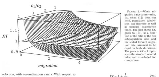
(12) holds even if subdivision is not geographic. We note that the effect of nonconservative migration in reducing genetic variability is not limited to fast mi- gration. Figure l illustrates this by plotting ET against

cl/% and the scaled forward migration rate, here as- sumed to be the same in both directions. It is clear that when the number of migrants is small, ET is sharply increased relative to its neutral value of one, whereas for large numbers of migrants, ET is smaller than one (except when cI/c2 = 1, which implies conservative mi- gration). The negative effect is stronger the more asym- metric the migration.

Most coalescent models of geographic subdivision have assumed conservative (and often symmetric) mi-

gration (TAKAHATA 1988; HUDSON 1990; HEY 1991;

HERBOTS 1994). Exceptions include the work of TAJIMA (1989) and of NOTOHARA (1990, 1993a,b), who also looked at the case of fast migration. The results of this section agree with those of the latter two authors.

As

shown in the APPENDIX, the expressions for the expected coalescence times under slow migration sim- plify considerably if migration is assumed to be conser- vative. They have a particularly simple form when the subpopulations are of equal size ( i e . , c1 = q = 1/2) so

that the model is completely symmetric. In this case, we have a single migration parameter m = bI2 =

bl.

It is easy to show that E n ( 2 , O)] = ET[(O,

2)]

= 1,

E n ( 1 , l ) ] = 1

+ -

1 ₍₁₃₎ 2M ’

and

1 4M ’

E T = 1

+

-

where M is the scaled migration rate 2Nm (SLATKIN 1987; STROBECK 1987; TAKAHATA 1988; TAJIMA 1989a;

HUDSON 1990; HEY 1991; NOTOHARA 1993a; HERBOTS

1994).

For future reference, we note that WRIGHT’S fixation index, Fsn can be calculated approximately from the painvise coalescence times as

where Eqw] is the average of the expected coalescence times for pairs of genes sampled within a subpopulation (SLATKIN 1991; HERBOTS 1994). For the symmetric model, where Eqw] = ( E n ( 2 , O ) ]

+

E n ( 0 ,

2)1)/2,

we thus have

1 1

+

4M’

F,,. =

-

in agreement with earlier results (WRIGHT 1951; NEI

1975; TAKAHATA 1983; CROW and AOKI 1984; SLATKIN

1991; HERBOTS 1994). Note that this result differs from the classical result FST = 1/ (1

+

4Nm) because the num- ber of demes here is two rather than infinite.

General selection model: Imagine a single popula- tion in which a two-allele polymorphism with alleles A I

and A2 has been maintained for a long time by some combination of selection and mutation (e.g., heterozy- gote advantage or mutation-selection balance) at fre- quencies

p

and q = 1

-

p.

Let uti be the mutation rate from A, to A,. The forces maintaining the polymorphism are assumed to be strong relative to random drift, so

Time Scales in the Coalescent 1505

1.

ET

0

migration

selection, with recombination rate r. With respect to this locus, the population can be subdivided into two allelic classes, because a given gene is linked either to an A , or an A2 allele. We can thus use the same model as for migration with q =

p ,

cz

= q, and transition probabilities given by

q(*1

+

P)

P

P(u12

+

gr)

b12 = ₍₁₇₎

b 2 1 =

,

(18)

to linear order in the recombination and mutation rates, as well as in the selection coefficients (HUDSON and KAPLAN 1988; KAPLAN et dl. 1988; HEY 1991).

Balancing selection: We first look at the case of bal- ancing selection (HUDSON and WLAN 1988; KAIJLAN

et al. 1988; HEY 1991). Note that if uii Q r, we have bI2

=

gr

and

=

p.

Since the mutation rate from one functional allele to another is likely to be extremely low, this will be true except for sites that are very tightly linked to the balanced polymorphism.

Assume first, therefore, that mutation is negligible. Under this assumption, 6

=

0, because recombination, as it is modeled here, is by itself always conservative in the sense of (12). If ris large, so that the fast approxima- tion is appropriate, we thus see immediately from (6)

and the accompanying argument that the balanced polymorphism has no effect (to the assumed order of approximation) on the coalescence process. If r is

O(

1 /A'), we define

4

lim 2Nr = (19)

and obtain the expected coalescence times precisely as for the case of geographic subdivision (the results are given in the APPENDIX). If the balancing selection is

symmetric, so that p = q = we have

E

n

(2, 0) ]

=

E q ( 0 , 2)] = 1, E n ( 1 , l ) ] = 1

+

l/R

and

I\ +

FIGURE 1.-When mi- gration is not conservative,

Z.P., when (12) does not hold, population subdivi- sion can decrease as well as increase coalescence times. The plot shows ET, given by ( l o ) , as a func- tion of the ratio of the two

subpopulation sizes and the scaled forward migra- tion rate, assumed to be equal in both directions. The plane at ET= 1 repre- sents the standard neutral value and is included for comparison.

1

2R'

E T = l + -

which should be compared with the results for the mi- gration model (HUDSON and KAPLAN 1988; KAPLAN et al. 1988; HEY 1991).

If mutation is not negligible compared with recombi- nation, there may be a negative effect on the coales- cence time that is not due to linkage, but to nonconser- vative flow between the allelic classes. Numerical studies indicate that this effect is negligible compared with the effect of linkage except when the b, are relatively large. For the biological reasons mentioned at the beginning of this section, however, the b, will never be large unless the u, are negligible compared with r. This negative effect should therefore never be important under bal- ancing selection.

Background selection: Now assume that the poly- morphism is maintained by mutation-selection balance instead of balancing selection. Let A , be the wild-type allele and A2 the (class of) deleterious ones, and define

wI1

= 1, wI2 = 1 - t , , and y2 = 1

-

ti, where the selection coefficients are assumed to be small as before. The deleterious mutation rate, uI2 = u, is also assumed to be small (although several orders of magnitude greater than u I 2 in the previous section), and the re- verse mutation rate, is assumed to be negligible. To the order of approximation, we thus have

b12 = gr,

1. This clearly implies that

b1

%= O( l/N), so we must use the fast approximation. As we have seen ($ the argument accompanying Equation 6), this is tanta- mount to saying that the effect of the selected locus on the coalescent at linked sites is equivalent to a reduction in the effective population size. The resulting decrease in expected variability is known as “background selec- tion” ( CHARLESWORTH et al. 1993). Using (1 1 ) we ob-

tain directly, to linear order in

q,

r, and t l ,

E T = l - !I (23)

(1

+

-$’

which is the result found by HUDSON and KAPLAN (1994, 1995) using a related coalescent approach, and by NORDBORG et al. (1996a) using diffusion methods.

For n loci in mutation-selection balance that interact multiplicatively, it has been argued that

where

qj,

ri, and tli are the parameters defined above for each of the n loci; Monte Carlo simulations indicate that this approximation is quite good (HUDSON and KAPLAN 1995; NORDBORG et al. 1996a). We note that an induction argument based on the single-locus result in this article also suggests the approximation given by (24), but that the validity of the time-scales approxima- tion as the number of loci increases and the frequency

of chromosomes free of deleterious mutations de- creases remains to be determined. We will return to this issue in DISCUSSION.

For future use we define a as the ratio of ET under background selection to ET without background selec- tion. Since the latter equals 1 when time is scaled in units of 2N, a is given by (24). Of course, (Y is equal to the 7r/7ro of CHARLESWORTH et al. (1993) and can also be interpreted as NJN, where N,is the effective popula- tion size under background selection.

MIGRATION AND SELECTION

To investigate how two different processes, such as migration and selection, jointly affect the coalescent, it is necessary to subdivide the population twice. Imagine, therefore, a Wright-Fisher population of size N diploid individuals, but this time divided into four classes of size N,, i = 1,

.

. .

, 4. As before, let b,, i,

j

= 1,

.

. .

, 4

be the probability that a given gene in class i was in class j in the previous generation. To describe the gene- alogy of a pair of genes, we now need a minimum of 11 states: the absorbing state plus

(2,

0, 0, 0 ) , (1, 1, 0, O ) , (1, 0 , 1, O ) , (1, 0 , 0 , I ) , ( 0 , 2, 0 , O ) , ( 0 , 1, 1, O ) , (0,

1, 0 , l ) , ( O , O , 2, O ) , (0, 0 , 1, 11, and ( 0 , 0 , 0 , 2), where

( k ,

I,

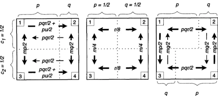
m, n) denotes the state with k distinct genes in the first class, I distinct genes in the second class, etc.

We are interested only in the special case of this model in which the four different classes are defined by two dichotomous criteria. For example, we may have geographic subdivision into two subpopulations com- bined with “genetic subdivision” into two allelic classes (Figure 2 ) . This restriction imposes two constraints on the general model. First, the size of each class can be found by multiplying the sizes of its class with respect to the two levels of subdivision (e.g., Nl = clpNin Figure

2 ) . Second, the probabilities of exchange between classes separated by two levels of subdivision (ie., b14, b41,

&3, and 6 3 2 ) will be smaller than the other probabilities. Three different combinations of time scales are of

interest. First, if the probabilities of exchange between the classes are O(l/N) on both levels ( L e . , horizontally and vertically in Figure

2),

we obtain an approximate process of the same dimensionality, analogous to the slow approximation described above. Second, if the rates of exchange are all high, the process reduces to a singledimensional one, analogous to the fast approxi- mation. As before, this single-dimensional process will be the usual coalescent on a different time scale. All that is needed to understand this process is thus de- termining the correct time scale (which may sometimes be algebraically difficult).

The third possibility is that flow across one level of subdivision is fast, whereas flow across the other is slow. This case can be analyzed using an obvious extension of the previously given arguments. Assume (without loss

of generality) that jumps between 1 and 2, and 3 and 4 (horizontal flow in Figure 2) occur at a high rate, whereas all other jumps occur with probability O(l/N) or less. Then a very large number of horizontal jumps will occur before any vertical jumps occur, and, on a continuous time scale with time measured in units of O(N) , vertical jumps will occur according to the station- ary states of three possible “horizontal” equivalence classes, namely

I = ((2, 0 , 0, O ) , (1, 1, 0, O ) , (0, 2, 0 , O ) ) , B = ((1, 0, 1, O ) , ( 1 , 0 , 0 , l ) , (0, 1, 1, O ) , (0, 1 , 0 , l ) ] ,

C = ((0, 0, 2, 0 ) , (0, 0, 1, l ) , ( 0 , 0, 0, 2)], (25)

which of course correspond to the states (2, 0 ) , (1, 1) and, (0,

2),

respectively, for the vertical process. Jumps between these states

(as

well as coalescent events) occur according to an exponential process on a time scale of

O(N), as usual. It can be shown that this process has a transition matrix that looks identical to the transition ma-

trix (2), except that By, i,

j

= l, 2 is replaced by l$, where

b12

B12

= ___ (B23

+

B24)

+

-

”

(B13

+

B14), (26)

m l

+

~ 3 (27) ~ ) ~

biz

+

b~

612

+

b 2 1

b34

&

=- _(B41

₊

_B42)

₊

~

643

634

+

643 b34

+

b43

Time Scales in the Coalescent 1507

P

9

4

+

p9r/2

-

4

Q!

E

.

Q . . .

I

p

=

1/2

9

=

1/2

"

.c.

P

9

9

P

FIGURE 2.-Examples of models with two levels of subdivision. The values on the arrows are biic,, i e . , they are proportional to the total number of immigrants; the parameters are defined in the text. From left to right, the models are as follows: migration and background selection, migration and balancing selection without local adaptation, and, finally, migration and balancing selection with local adaptation.

Since the real subpopulation sizes for the slow, vertical process are cl

+

q and c3

+

c4, it is clear that the fast, horizontal process will act to reduce these unless the fast flow is conservative. Coalescent events may there- fore occur at a faster rate within each subpopulation. It does not seem possible to say anything equally general about the effect of the fast process on the Bi, making the effect on the total coalescence time hard to predict. General selection-migration model: We begin by combining the models of geographic subdivision and

P , m

P,

0

selection introduced above. Let

pi(

qJ be the frequency of A,(A2) in subpopulation i. The mutation rates are assumed to be the same in the two subpopulations, but the selection coefficients may differ (which may lead to differences in allele frequencies between the subpopu- lations). For clarity, we restrict our attention to the case of conservative symmetric migration (Le., equal subpop ulation sizes and a single migration rate m)

.

The critical parameters are the bi, ofwhich there are now 16 (rather than the two needed for one level of structure). They can be found through standard population genetics theory, but are of course quite complicated in their exact form, and depend on the details of the life cycle assumed. However, using the same approximations as before, it can be shown that, to linear order in migra- tion, selection, recombination, and mutation, the b, are the elements of the matrix

0

Pl

0 _. 42m

Q1

Migration and background selection: First assume at equilibrium must be equal, as depicted in the left that the polymorphism is maintained by mutation-selec- panel of Figure

2.

Thus, we have

p,

= P, =

p

and q1 =

tion balance with parameters as in the previous section. ₄₂ = q in the matrix (30).

O( 1/N), so that we have the combined fast-slow process we just described. It is obvious that C, =

4

and

BIZ

=

&

because of symmetry. This observation alone gives us E n ( 2 , O)] = ET[(O, 2)] = 22, and

where the states ( k , I ) refer to the geographic subdivi- sion. Since the modified subpopulations are of equal size, we also have

1

ET = 2 4

+

7

4 4

It is easy to show that

and that

8v

= M , i, j = 1,

2,

(34)

where M, as before, is the scaled migration rate 2Nm. To the order of approximation, background selection affects only the effective subpopulation sizes, not migra- tion between subpopulations.

Generalizing to multiple loci in mutation-selection balance, we have Enw] a , and

1

4M ’

E T ~ c Y + - _{( 3 5 )}

where a is still given by (24).

As

a consequence, the relative amount of time spent between subpopulations is increased, so that

1 1 + 4Ma

FS, M

Background selection thus leads to an apparent in- crease in population differentiation, as conjectured by

HUDSON and KAPLAN (1995). For completeness, we note that the case of high migration is trivial (just let

M -+ 00 in all expressions).

Balancing selection and background selection: Imag- ine that the locus under study is linked to a balanced polymorphism on one side with recombination rate r and to a locus in mutation selection balance on the other side with recombination rate

7‘.

It is easy to see that, under the assumptions used throughout this paper

(notably the assumption that double recombination events are negligible), this model is identical to the one of the previous section if we replace population subdivision with balancing selection. If the allele fre- quencies for the balanced polymorphism are equal, for example, we have

E T = 1 -

+ -

1

( 1

+

7‘/t1)‘ 2 R ’ (37)

and for the case of multiple loci in mutation selection balance, we would have

1 2R

’

E T = a + -

as conjectured by NORDBORC et al. (1996b).

Migration and local adaptation: We now return to the general model of migration and selection and as- sume that the genetic polymorphism is maintained by some form of local adaptation instead of by mutation- selection balance. To the order of approximation, the resulting model is identical to the more general model of balancing selection in a subdivided population stud- ied by KAPLAN et al. (1991). These authors did not, however, derive the results for strong local adaptation that will be given below.

Assume that the genetic polymorphism is maintained by local adaptation with negligible mutation between the two alleles. Directional selection favors AI over A2

in the first subpopulation, and A2 over AI in the second. We wish to contrast this situation with one in which the overall allele frequencies are the same, but do not differ between the subpopulations (i.e., there is some form of balancing selection without local adaptation, or the degree of local adaptation is very weak). For simplicity, we will assume that the overall allele frequencies are equal, i.e.,

pl

+

pr

=

q1

+

q2 = For this to be the case, the local adaptation must be symmetric so that

PI

= q2 =

p

and q1 =

p,

= q, as depicted in the right panel of Figure 2. Note that the case of weak or no local adaptation can be obtained from this model simply by letting

p

= q = as depicted in the middle panel of Figure 2.

Local adaptation is similar to background selection in many ways. Within each subpopulation, polymor- phism is maintained by migration-selection balance, just as it is maintained by mutation-selection balance under background selection. If the migration rate is low, we will have

q

=

m/ tl, where tl is the selection

coefficient against heterozygotes (HALDANE 1930).

Thus, for the allele frequencies

p

and

q

to be constant, we need to assume that m

>

O(l/N), so that only the fast approximation for migration is appropriate [the case of slow migration requires a different argument

(M. NORDBORG, unpublished data)]. N o such restric- tion applies if the genetic polymorphism is maintained by some other form of balancing selection, nor, obvi- ously, to the rate of recombination.

If recombination and migration are both slow (again, this case is not applicable when the polymorphism is maintained by strong local adaptation), we find the expected coalescence time for each of the 10 possible initial states as before (see APPENDIX). The mean coales- cence time within subpopulations is

1 1

E n w , subpopulation] = 1

+

-

+

2R 4M

+

2R’

.

(39)

Time Scales in the Coalescent 1509

1 1

E n w , allelic class] = 1

+

-

+

4M 4 M + 2 R '

and that for a random sample, finally, is

1 1 1

E T = l + - + - +

4M 2R 4 M + 2 R ' (41)

If recombination and migration are both fast, we use the fast-fast approximation. Because of the high degree of symmetry in the transition matrix, it is possible to find the relevant effective population size explicitly. It can be shown that

Without local adaptation,

p

=

q

and ET = 1, whereas if local adaptation is strong we have m

=

qtl, q small, and

(42) can be approximated by

E T = 1 -

(1

+

r/tl)* ' (43)

which is identical to (23). Thus, local adaptation speeds up the coalescent by decreasing Ne at sites linked to the selected locus, an effect analogous to that of back- ground selection.

This is only true when ris of the same order of magni- tude as m, however. For closely linked sites, i.e., when

r is O(l/N), we must use the fast-slow approximation instead. Note that, in terms of Figure 2, the vertical process is now fast, and the horizontal one slow, so the indices on the right-hand side of (26) - (29) must be changed in the appropriate manner. This done, the expected coalescence times in terms of the

Bi,

and are the same as for background selection and geographic subdivision. In the present case, however, we have

and

(45)

Thus, if there is no local adaptation,

p

= q = 1/2 and

the expected coalescence times are identical to those obtained for balancing selection without geographic subdivision. Under strong local adaptation ( i e . , q

small), on the other hand, we have

and

1

- q

+ -

(47) 2qR

1

4'-. (48)

4qR

Thus, the effective allelic class size is decreased by the migration-selection balance. The major effect of local adaptation, however, is to reduce the effective recombi- nation rate, because heterozygotes are uncommon

(KAPLAN et al. 1991). We note that the approximations given by (42) -(43) and (48) are consistent with each other, because large Rin the latter corresponds to small T in the former, and the approximations converge to

What about Fs, under this model? Because the rate of migration is assumed to be high, one might expect that FsT = 0. This is indeed the case when there is no local adaptation

(p

= q) and also when FST is measured within allelic classes. If FST is measured in the normal

fashion (i.e., without regard to allelic classes), however, we have

1 - q.

ET[

w, subpopulation] = P E T [ (2, 0 ) ]

+ 2pqEn (1, 1

) ]

so that

1

1

+

4qR '

FST ~

where the approximations apply for small q, as before. Thus regions of the genome close to polymorphic sites maintained by migration-selection balance may exhibit extremely high FST values even though FST for unlinked

sites is zero.

INCORPORATING SELFING

It has recently been shown that the standard coales- cent can be extended to incorporate partial selfing by simply keeping track of whether genes are in the same or different individuals and noting that the time spent in states involving two genes in the same individual is negligible on the coalescent time scale (NORDBORG and

where s is the fraction of offspring produced by self- fertilization, i e . , the selfing rate. This result is in agree- ment with the classical result (LI 1955; WRIGHT 1969; POLLAK 1987), often written

1 l + F

N, =

-

_N,

where F = s/ (2 - s) is the equilibrium inbreeding coef- ficient for a neutral locus (HALDANE 1924). In the re- mainder of this section, I will use this insight to show how partial selfing affects models of migration or selec- tion.

Selfing and migration: This case is straightforward. The time until the ancestors of two genes in different subpopulation are found in the same subpopulation is unaffected, but the rate at which two genes in the same subpopulation coalesce is increased by a factor 1

+

F, as we just have seen. For the completely symmetric two- deme model, we have E T [ w] = 1/ (1

+

r;) and

1 1

l + F 4M

E T = - + - .

Clearly,

(53)

(54)

Selfing will thus always increase FS,. Note the analogy between the effects of background selection and selfing: both act to decrease N, and therefore affect the coales- cence times in the same way. Note also that if migration occurs via pollen flow, the migration rate would of course be directly affected by the degree of selfing. This is not the case for diploid migration.

General selection model with selfing: If extending the model of geographic subdivision to incorporate selfing is trivial, extending the model of subdivision into allelic classes is considerably less so. The reason for this is that whereas migration is assumed indepen- dent of genotype, recombination is not, because it can only take place in heterozygotes. This is, of course, true with random mating as well, but does not cause a prob- lem because, under random mating, the probability that the parent of a given gene was a heterozygote does not depend on the genotype of the individual in which the gene resides in the current generation. With selfing, this is obviously not true, and we therefore need to divide the population into genotypic as well as allelic classes. For example, a gene in the first allelic class (it?.,

linked to an A I allele) is either in the AlAl or the AIA2 genotypic class. Since, under partial selfing, we also need to keep track of whether two genes are in the same individual or not, 13 states (plus the trivial ab-

sorbing state) are needed to model the genealogy of a pair of genes as a discrete-time Markov process. This should be compared with three states under random mating.

Fortunately, it is possible to completely eliminate these extra dimensions by appealing to separation of time scales. As before, coalescent events occur on a time scale that is O(N), and jumps between the allelic classes

(ie., recombination and mutation) occur on a time scale that is either O(N) or much faster. What about jumps between the genotypic classes? These are caused by Mendelian segregation and occur with very high probability per generation. We thus introduce a third time scale to describe these jumps, and simply argue that the process will have reached stationarity with re- spect to the genotypes long before any other jumps

(due to recombination, mutation, or coalescence) take place. Let x,

y,

and z be the equilibrium frequencies of the three genotypes A I A I , AIA2, and A2A2, respectively. These frequencies will be constant to the assumed order of approximation. The stationary probability that a gene linked to an A, allele is in a heterozygote is y/ (2x

+

y), otherwise it is in a homozygote ( A I A , ) . The analogous probability for a gene in the second allelic class is of course y/(2z

+

y). Using these stationary probabilities, and the same approximations as for ran- dom mating, the transition probabilities governing jumps between allelic classes can be shown to be

where 7 = (1 - f i r . These equations should be com- pared with

(17)

-

(18). Selfing always affects the b, by reducing the effective recombination rate, and possibly also by altering the equilibrium values of

p

and

q.

Selfing and balancing selection: Given this result, the case of balancing selection is simple. As before, we ig- nore mutation. Jumps between allelic classes occur as before, but at a rate that is reduced by a factor 1 - F. Coalescence events within allelic classes occur at a rate that is increased by a factor 1

+

F. The results obtained for random mating hold with straightforward modifica- tions. For example, in the case

p

= q = we have E n w , allelic class] = 1/(1

+

4,

and

1 1

1 + F 2 R '

E T =

-

+

--

(57)

where

R

= (1 - r;) R, as conjectured by NORDBORC et

al. (1996b).

Time Scales in the Coalescent 1511

q p

P

4

f

? + - U

otherwise it is in the class of wild-type alleles (;.e., A I ) . Coalescent events occur within these two classes with rates (1 + f l / q and (1

+

q / p ,

respectively. Define

2

=

(1 -

t)

tl

+

Fk. Under the assumption that the deleteri-

ous allele is rare

(6

HALDANE 1927), we then obtain

q

M u/f directly from the genotypic recursions. Using this and the same approximations as before, it is easy to show that

This expression should be compared with (23).

Analogously to the case of random mating, we conjec- ture that the effect of ?z loci in mutation-selection bal-

ance can be approximated by

and redefine a to be NJN, where N, is the effective population size under background selection and selfing (given directly by Equation 60; $ the discussion follow- ing Equation 24).

MIGRATION, SELECTION, AND SELFING

This section illustrates how all the forces discussed in this paper act in combination, by extending the model of balancing selection in a subdivided popula- tion to include partial selfing and background selec- tion. The results for the simpler models can be recov- ered as special cases.

No local adaptation: We first look at the case of a balanced polymorphism maintained by symmetric se- lection acting independently of population subdivision

($ Figure 2, middle panel).

As we have seen, background selection and selfing act to reduce the expected coalescence time within s u b populations and allelic classes. Selfing decreases the rate of exchange between allelic class by a factor 1

-

F, and neither process affects migration. Equations 39-

41 thus become

1 1

ET[w, subpopulation]

=

a

+

7

+

2R 4 M + 2 R ’ (61)

and

ET[w, allelic class]

=

a

+

- 1

+

1

4 M 4 M +

2 R ’

(62)

1 1 1

E T = a + - + - +

4M 2R 4 M + 2 R ’ (63)

The results for fast migration or recombination can be obtained by letting the relevant parameter go to infinity.

It is easy to show that Fvequals 1/( 1

+

4Ma) for unlinked loci but is affected by R otherwise. The

FST

statistic can also be used to with respect to the allelic classes as

E T - E q w , allelic class]

E T 2 (64)

in which case it, loosely speaking, measures the fraction of the total variability that is due to the division into allelic classes. For high migration, this measure equals

1/(1

+

2aZ?), which shows that balancing selection has much greater effect on variability in the presence of selfing and background selection (NORDBORG et al. 1996b).

Local adaptation: The local adaptation model ($

Figure 2, right panel) can be treated similarly. For sites that are tightly linked to the selected locus, E n w , allelic class]

=

a ( l - q ) ,

1

R ’ E n w, subpopulation]

=

a

(1 -

q)

+

X (65)

and

In this case, FS, is approximately equal to

regardless of whether it is measured with respect to subpopulations or allelic classes (this is so because al- leles are so strongly correlated with subpopulation). Since recombination is weighted by a factor 4 p ( 1 -

a,

which may be very small, it is clear that high Fv values may be expected even for loosely linked sites.

DISCUSSION

This article has demonstrated how arguments based

tion. Below, I discuss the main results and their implica- tions.

Fast processes and Ne: The central point of this arti- cle is that any process that effectively subdivides the population into a number of classes connected by fast flows ( i e . , transition probabilities much greater than

0(1/N) per generation) can be modeled simply as a change in

Ne.

This result is not limited to a sample size of two. Examples include geographic subdivision with high migration rates, background selection, and partial selfing. Arguments based on separation of time scales in the coalescent have been used before (KAPLAN et al. 1991; TAKAHATA 1991), but not presented as a general approach.

Because the concept of Ne is perhaps more commonly used than understood, it is worth belaboring what this result means. By saying that a certain population struc- ture can be modeled as a change in Ne, I mean that an appropriate change in the coalescent time scale will retrieve the equivalent unstructured coalescent process, allowing standard analytical results and software to be

used (DONNELLY and TAVAR~ 1995; NORDBORG and

DONNELLY

1997). This claim is much stronger than, for instance, the statement that the expected coalescence time for a sample under a certain model of population struc- ture is equivalent to that of an unstructured population of some effective size (NEI and TAKAHATA 1993).

Nonconservative migration: When the flow in a structured coalescent is nonconservative, expected co- alescence times may be decreased by subdivision as well as increased (cf: Figure 1). Indeed, if the flow is fast, the expected coalescence time will always be reduced, an effect equivalent to a decrease in Ne (NAGW 1980;

NOTOHARA 1993a).

It is easy to see why population structure can increase the total coalescence time, because two genes in differ- ent subpopulations cannot coalesce until a migration event brings them to the same subpopulation, but what is the intuition behind the decreased coalescence time under non-conservative migration? When (12) does not hold, there is a net gene flow from one subpopulation to the other. Looking forward in time, a parent in the “upwind” (net donor) subpopulation is more likely to leave offspring than a parent in the “downwind” (net recipient) subpopulation. Looking backward in time, the ancestor of a gene in the downwind population is more likely to have lived upwind than the other way around. Clearly this may cause a reduction in N,, and, therefore, shorter expected coalescence times.

In the real world, we would often expect migration to be nonconservative, however, most theoretical analy- ses of subdivided populations have assumed the sim- plest version of the finite island model, in which migra- tion is both symmetric and conservative. The results from this model are widely used and quoted, yet their robustness to violations of these basic assumptions do not seem to have been investigated.

Background selection: As we have seen, background selection can be interpreted as a form of nonconserva- tive, fast migration. In this case the heuristic explana- tion just given works even better because “wind” is explicitly included in the model in the form of the (unidirectional) deleterious mutation rate. It should thus be possible to model background selection simply as a reduction in Ne, but this conclusion is contradicted by the negative values of TAJIMA’S D statistic seen in simulations of this process (CHARLESWORTH et al. 1993, 1995; HUDSON and -LAN 1995): if a reduced Ne was the only effect of background selection, TAJIMA’S D should have a mean value of zero (TAJIMA 1989b).

This apparent contradiction is resolved by realizing that the extension of the single-locus result to multiple loci is not rigorous. In particular, a random sample from a population will not be drawn according to the stationary distribution of the fast mutation-recombina- tion process. Under the single-locus background selec- tion model, a randomly sampled gene will be linked to a deleterious mutation with probability q, whereas the stationary probability is b I 2 / ( b l 2

+

bl)

=

q/ (1 + t l / r ) . This difference will disappear instantly on the coales- cence time scale, and can thus be ignored. With multi- ple loci, however, it is possible that convergence to the stationary state could be slow enough to be detected, especially for large sample sizes and values of

8,

which is precisely the circumstances under which significant negative TAJIMA’S D have been observed (CHARLES- WORTH et al. 1995).

There are further inaccuracies associated with the approximations for multilocus background selection. Monte Carlo simulations have shown that whereas (60)

is quite accurate for random mating (CHARLESWORTH

et al. 1993; HUDSON and KAFTAN 1995), it is considerably less accurate for selfing populations

(B.

CHARLES WORTH, M. NORDBORG and D. CHARLESWORTH, u n p u b lished data). Furthermore, simulation of models that include balancing selection

(NORDBORG

et al. 1996b)

and migration (B. CHARLESWORTH, M. NORDBORG and

D. CHARLESWORTH, unpublished data) indicate that the statement that background selection only affects the coalescence time within classes (e$ Equations 35 and 38) is only correct to a rough approximation for strong background selection.

Time Scales in the Coalescent 1513

either in the form of selective sweeps

(IMAYNARD

SMITH

and HAIGH 1974; -LAN et al. 1989), or in the form of background selection (CHARLESWORTH et al. 1993), levels of variability may easily be reduced by several orders of magnitude, dwarfing the twofold reduction due to inbreeding (CHARLESWORTH et al. 1993; NORD-

BORG et al. 1996b). Similarly, if selection acts to maintain a given polymorphism in a selfing species, a much larger region of the genome will be affected, a point to which we will now turn.

Detecting selection: The action of balancing selec- tion may be detected because it leads to a peak of vari- ability surrounding the selected site (KREITMAN and

AGUADE 1986; HUDSON and 1988; KAPLAN et al. 1988). The results of this article suggest three situations when such a peak may be easier to detect. First, selfing will increase the size of the region affected. Second, any background selection should decrease the variabil- ity within each allelic class, making the peak much more apparent. This may be especially relevant in a selfing population where the effect of background selection is expected to be considerable (NORDBORG et al. 1996b). Third, if a balanced polymorphism is maintained by local adaptation ( i e . , in a cline), the peak will also be much wider. Under the right conditions, it may even be possible to scan the genome directly for such poly- morphisms.

Apparent subpopulation differentiation: The pres- ent results also show that population subdivision may be severely overestimated under some conditions. Because both selfing and background selection decrease coales- cence times within subpopulations, they will inflate FST values. This is, of course, consistent with the notion that

Fyr depends on Npm, but it nonetheless implies that it is impossible to draw conclusions about isolation from this statistic. If, for example, background selection or selective sweeps were to reduce variability by a factor of 100, Fs7. would behave as if the migration rate was one- hundredth of its actual value.

Another concern is linkage to polymorphisms main- tained by local adaptation in a cline.

As

shown by (67),

Fyr values will be extremely inflated in a region sur- rounding such loci, and, especially for organisms with a high natural rate of self-fertilization, this region may be quite wide. Indeed, very high Fyrvalues and extensive allozyme linkage disequilibria have often been found in highly selfing plants (e.&, HAMRICK and GODT 1990 and other contributions in the same volume). The re- sults presented here suggest a simple interpretation for these observations.

I thank B. CHARLESWORTH and D. CHARLESWORTH for suggesting the model studied in this article and for continual discussions. I am very grateful to T. NAGYIAKI for patiently explaining some of the intricacies of migration theory, as well as for extensive commentS on the manuscript. The manuscript also benefited from the comments of P. DONNELLY, R. R. HUDSON and an anonymous reviewer. This work was supported by National Science Foundation (NSF) grant

DEB-9217683 to D. CHARLESWORTH and by NSF grant DEE9350363 to J. BERGELSON.

LITERATURE CITED

CHARLESWORTH, B., M. T. MORGAN and D. CHARLESWORTH, 1993 The effect of deleterious mutations on neutral molecular varia- tion. Genetics 134 1289-1303.

CHARLESWORTH, D., B. CHARLESWORTH and M. T. MORGAN, 1995 The pattern of neutral molecular variation under the back- ground selection model. Genetics 141: 1619-1632.

CROW, J. F., and K. AOKI, 1984 Group selection for a polygenic be- havioral trait: estimating the degree of population subdivision. Proc. Natl. Acad. Sci. USA 81: 6073-6077.

DONNELLY, P., and S. TAV&, 1995 Coalescents and genealogical structure under neutrality. Annu. Rev. Genet. 29: 401-421. HALDANE, J. B. S., 1924 A mathematical theory of natural and artifi-

cial selection. Part 11. Proc. Camb. Phil. Soc., Biol. Sci. 1: 158- 163.

HALDANE, J. B. S., 1927 A mathematical theory of natural and artifi- cial selection. Part V Selection and mutation. Proc. Camb. Phil. SOC., Biol. Sci. 23: 838-844.

HALDANE, J. B. S., 1930 A mathematical theory of natural and artifi- cial selection. Part VI: Isolation. Proc. Camb. Phil. SOC., Biol. Sci.

HAMRICK, J. L., and M. J. GODT, 1990 Allozyme diversity in plant species, pp. 43-63 in Plant Population Genetics, Breeding, and Ge- netic Resources, edited by A. H. D. BROWN, M. T. CLEGG, A. L.

KAHI.ER and B. S. WEIR. Sinauer Associates, Sunderland, MA.

HERBOTS, H. M., 1994 Stochastic Models in Population Genetics: Geneal- o g ~ and GeneticDijfwentiation in Structured Populations. Ph.D. thesis, University of London.

HEY, J., 1991 A multidimensional coalescent process applied to multi-allelic selection models and migration models. Theor. Po- pul. Biol. 3 9 30-48.

HUDSON, R. R., 1990 Gene genealogies and the coalescent process, pp. 1-43 in Oxford Surveys in Evolutionaly Biology, edited by D. FUTLW and J. ANTONOVICS. Oxford University Press, Oxford. HUDSON, R. R., and N. L. KAPLAN, 1988 The coalescent process in

models with selection and recombination. Genetics 120: 831- 840.

HUDSON, R. R., and N. L. KAPLAN, 1994 Gene trees with background

selection, pp. 140-153 in Nan-Neutral Evolution: Theories and M w lecular Data, edited by G. B. GOI.DING Chapman & Hall, New York.

HUDSON, R. R., and N. L. KAPIAN, 1995 Deleterious background selection with recombination. Genetics 141: 1605-1617. KAFTAN, N. L., T. DARDEN and R. K. HUDSON, 1988 The coalescent

process in models with selection. Genetics 120: 819-829.

KAPIAN, N. L., R. R. HUDSON and M. I I ~ U K A , 1991 The coalescent

process in models with selection, recombination and geographic subdivision. Genet. Res. Camb. 57: 83-91.

KAPL\N, N. L., R. R. HUDSON and C. H. LANGLEY, 1989 The “hitch- hiking” effect revisited. Genetics 123: 887-899.

-ITMAN, M., and M. AGUADE, 1986 Excess polymorphism at the

Adh locus in Drosophila melanogaster. Genetics 114: 93-110. KREITMAN, M., and H. AKASHI, 1995 Molecular evidence for natural

selection. Annu. Rev. Ecol. Syst. 26: 403-422.

LI, C. C., 1955 Population Genetics. University of Chicago Press, Chi- cago.

MARUYAMA, T., 1977 Stochastic Problems in Population Genetics.

Springer-Verlag, Berlin.

MAYNARD SMITH, J., and J. HAIGH, 1974 The hitchhiking effect of a favourable gene. Genet. Res. 23: 23-35.

NAGYLAKI, T., 1980 The strong-migration limit in geographically structured populations. J. Math. Biol. 9: 101-114.

NEI, M., 1975 Molecular Population Genetics and Evolution. American Elsevier, New York.

NEI, M., 1987 Molecular Evolutionaly Genetics. Columbia University Press, New York.

NEI, M., and N. TAIWHATA, 1993 Effective population size, genetic diversity, and coalescence time in subdivided populations. J. Mol. Evol. 37: 240-244.