HERRING, NICHOLAS FRANKLIN. Ray Effects Mitigation in SN Problems through General Collision Monte Carlo Coupling and Numerical Validation of the THOR SN Code for Nuclear Nonproliferation Applications. (Under the direction of Dr. Yousry Azmy).
Discrete ordinates (SN) methods allow for computationally efficient solutions to radiation
transport problems. However, SN transport problems can suffer from a numerical phenomenon in
their solution called ray effects. This problem occurs during the propagation of radiation in low
in-group scattering regions far away from a localized source. Air is one low in-group scattering
medium due to its small optical thickness. This unfortunately means that ray effects are common
in nonproliferation applications since air regions are common in these problems. A proposed
approach for mitigating ray effects is to simulate the first few collisions of a transport problem
using a Monte Carlo method (which does not require any discretization but may be
computationally expensive) and using the results of that simulation as a source for the SN
calculation. This “few-collided source” is expected to be distributed more uniformly in space and
should lead to an SN transport solution that exhibits less ray effects.
Through coupling the SN code THOR (Tetrahedral High Order Radiation transport code)
with the Monte Carlo code Hammer, promising results in the practical application of this method
in systems which are not too highly scattering are obtained in this work. The method involves
evaluating low collision-count scattered flux with Hammer while the higher scattered solution is
calculated using THOR for a total flux solution obtained by combining the two results. Results
show the coupling to be effective in removing visible ray effects from the solution of a test
problem. Further analysis of the mitigation is performed on a simplified version of a real
experimental model to establish that accurate detector responses can be computed using our new
provide a benchmark problem for nonproliferation focused transport codes. Such a problem also
serves as a numerical validation for the THOR code in nonproliferation detector-based
applications. The specific model employed here is a simplified version of the full physical
experiment configuration. This simplification is done so we can rely more on coarser cells,
which allows for more computationally efficient calculations and allows us to resolve small
features that can be difficult to accurately model using tetrahedral meshes.
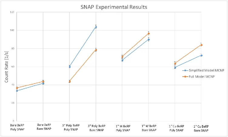
The calculation resulted in a full model continuous energy MCNP result within 20% of
the experimental count rates. Using the simplified model with multigroup cross sections gave
results within 40% of the continuous energy count rate, indicating a large error introduced by our
cross sections. Finally, the coupled Hammer and THOR results were less than 11% different
from the multigroup MCNP calculations. These results were even better for a model not
featuring the optional SNAP shield where they showed agreement to within 3% of the
multigroup MCNP results. This result was an improvement from the accuracy obtained with the
non-coupled THOR calculation which was only within 52% of the multigroup MCNP, indicating
© Copyright 2018 by Nicholas Herring
Ray Effects Mitigation in SN Problems through General Collision Monte Carlo Coupling and Numerical Validation of the THOR SN Code for Nuclear Nonproliferation Applications
by
Nicholas Franklin Herring
A thesis submitted to the Graduate Faculty of North Carolina State University
in partial fulfillment of the requirements for the degree of
Master of Science
Nuclear Engineering
Raleigh, North Carolina
2018
APPROVED BY:
_______________________________ _______________________________ Dr. Yousry Y. Azmy Dr. John Mattingly
Committee Chair
BIOGRAPHY
Nicholas Herring was born in Greensboro, North Carolina to James and Anita Herring.
He was homeschooled by his parents all throughout middle school and high school. After high
school, he attended North Carolina State University (NC State), where he obtained a BS in
nuclear engineering. His education continued at NC State for graduate school in nuclear
ACKNOWLEDGMENTS
First and foremost, my thanks go to my advisor, Dr. Yousry Azmy. He has guided me
through the thesis process and has been a major influence on the direction and style of my
research for the work described here. In addition, I appreciate the willingness of Dr. John
Mattingly and Dr. Robert Hayes to serve on my committee. I would particularly like to mention
Dr. Mattingly’s involvement in the experimental aspects of my thesis as he secured the ability for
us to perform the experiments on the Beryllium-Reflected Plutonium (BeRP) Ball. Staff at Los
Alamos National Laboratory and the Nevada National Security Site have proved invaluable in
securing the permission and training required to preform our experiments as well as model info,
in particular Jesson Hutchinson has provided much needed schematics and experimental
information. Dr. Sebastian Schunert at Idaho National Laboratory and Raffi Yessayan at North
Carolina State University have also provided invaluable assistance in understanding and
effectively applying the THOR transport code that much of this work relies on. The work
regarding the Monte Carlo code Hammer was performed by Dr. Brian Kiedrowski’s team at the
University of Michigan, so my appreciation extends to him and his team as well. I would also
like to thank the Integrated University Program Graduate Fellowship for financially supporting
my work as a graduate student and allowing me to pursue research topics of my interest. Finally,
I would like to thank CNEC for providing this problem and for partially funding this work for
TABLE OF CONTENTS
LIST OF TABLES ... vi
LIST OF FIGURES ... vii
Chapter 1: Introduction ... 1
Chapter 2: Review of Related Work ... 6
Neutron Transport Methods ... 6
Transport Theory and Equation ... 6
Monte Carlo Simulations ... 9
Hammer... 11
Discrete Ordinates ... 12
THOR ... 15
Ray Effects ... 16
Description of Effects ... 16
Mitigation Through Special Quadrature Sets ... 20
Mitigation Through Spherical Harmonics Equivalence ... 22
Mitigation Through Semi-Analytic Method ... 24
Mitigation Through Point-Kernel Method ... 26
Mitigation Through Monte Carlo Coupling ... 28
BeRP Ball Experiment ... 31
BeRP Ball Experiments ... 31
Experimental Models ... 34
Chapter 3: Experimental Campaign ... 36
Experiment Setup ... 36
Experiment Results ... 39
Chapter 4: MCNP Model Validation ... 41
Full Model of the BeRP Ball and the SNAP Detector ... 41
Validation of the Full Model and Error Quantification ... 43
Simplified Model of the BeRP Ball and the SNAP Detector ... 46
Numerical Validation of the Simplified Model and Error Quantification ... 49
Chapter 5: Coupled Model Development ... 53
Subcritical Multiplication for External Source Problems ... 53
Flux Visualization Method ... 56
Mesh Generation Method using SolidWorks ... 59
Converter from UNV format to THOR Mesh... 60
Boundary Conditions ... 61
Material Tracking... 61
SERPENT Cross Section Generation ... 62
Multigroup Cross Section Format Converter ... 63
Hammer to THOR Coupling Method ... 63
General Collision-count MC/SN Coupling Derivation ... 64
Practical Hammer-THOR Coupling Method ... 67
BeRP Ball in a Box Model... 68
Multigroup Cross Sections Generated by SERPENT ... 69
THOR Mesh ... 70
BeRP with SNAP Model ... 71
Multigroup Cross Sections Generated by SERPENT ... 71
Simulation with Multigroup MCNP ... 71
THOR Mesh ... 73
Hammer Model ... 75
Chapter 6: Computation Results and Numerical Validation ... 77
BeRP Ball in Air Test Problem: Mitigation of Ray Effects ... 77
Varying Quadrature Order in Pure SN Calculation ... 78
MC and SN Coupling ... 82
BeRP Ball with SNAP Detector: Numerical Validation... 87
Varying Quadrature Order in Pure SN Calculation ... 88
MC and SN Coupling ... 90
Chapter 7: Conclusions ... 97
Experiments ... 97
Model and Method Development ... 97
Computation Results ... 100
Numerical Validation of Method for Nonproliferation Applications ... 102
Potential Topics of Further Investigation ... 104
Streamlining the Method’s Implementation ... 104
Analysis of the Method’s Computational Costs ... 105
Tetrahedral Mesh Runs in MCNP ... 106
Better Energy Group Representation ... 106
Anisotropic Scattering Calculations ... 106
Experimental Validation ... 107
Multi Direction Coupling ... 108
Application for Reflected BeRP Ball ... 108
LIST OF TABLES
Table 2.1 Isotopic Composition of BeRP Sphere in 1980 ... 32
Table 2.2 Estimated BeRP Sphere Composition in 2009 ... 32
Table 3.1 Experimental Results from the SNAP Detector ... 39
Table 3.2 Experimental results from the MC-15 detector ... 40
Table 4.1 Spontaneous Fission Neutron Production Rate of BeRP Ball ... 42
Table 4.2 MCNP Results for the Full SNAP Model ... 44
Table 4.3 Simplified SNAP Dimensions ... 48
Table 4.4 Error introduced by simplifications to the full model ... 50
Table 4.5 Simplified Model Count Rates Computed by MCNP ... 51
Table 5.1 Multigroup MCNP vs Continuous-energy MCNP comparison ... 73
Table 5.2 Simplified Model Meshing Information without the HDPE SNAP Shield ... 73
Table 5.3 Simplified Model Meshing Information with the HDPE SNAP Shield ... 74
Table 6.1 SN Count Rates for the BeRP Ball and SNAP without the HDPE Shield and ARE Relative to the Multigroup MCNP Value in Table 5.1. ... 88
Table 6.2 SN Count Rates for the BeRP Ball and SNAP with the HDPE Shield and ARE Relative to theMultigroup MCNP Value in Table 5.1 ... 89
Table 6.3 Coupled Hammer-THOR Results for the BeRP Ball and SNAP without the HDPE Shield and Fission Enabled ... 90
Table 6.4 Coupled Hammer-THOR Results for the BeRP Ball and SNAP without the HDPE Shield and Fission Disabled ... 91
LIST OF FIGURES
Figure 2.1 Monoenergetic Ray Effects in Discrete Ordinates Solution ... 18
Figure 2.2 Point-Kernel Method ... 27
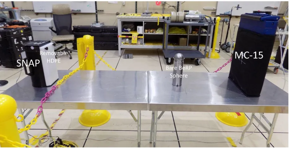
Figure 3.1 Bare BeRP Ball experiment with optional polyethylene shield attached to the SNAP detector ... 37
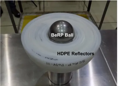
Figure 3.2 BeRP ball in the lower half of the HDPE reflector ... 38
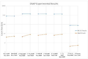
Figure 3.3 SNAP and MC-15 Results ... 40
Figure 4.1 Pu240 Spontaneous fission spectrum normalized over 20 MeV ... 43
Figure 4.2 MCNP vs Experimental Count Rates for SNAP detector ... 44
Figure 4.3 Absolute Relative Error with respect to the measured values in SNAP’s Count Rates Computed by MCNP Simulations Using the Full Model ... 45
Figure 4.4 Simplified SNAP Detector Model in SolidWorks ... 47
Figure 4.5 Simplified Experimental Model in SolidWorks ... 49
Figure 4.6 Comparison of Simplified and Full Model Count Rates ... 52
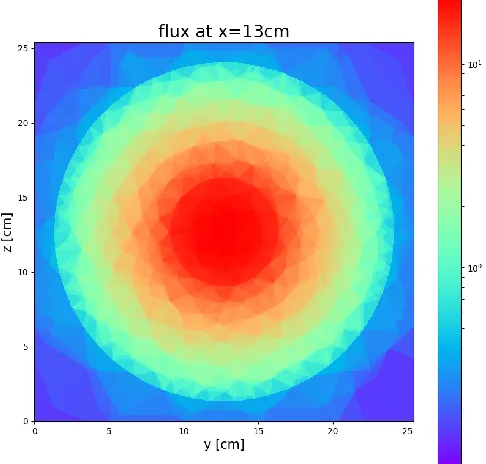
Figure 5.1 Fast flux plotted using option 1 of the visualizer for the BeRP Ball in HDPE Shell ... 57
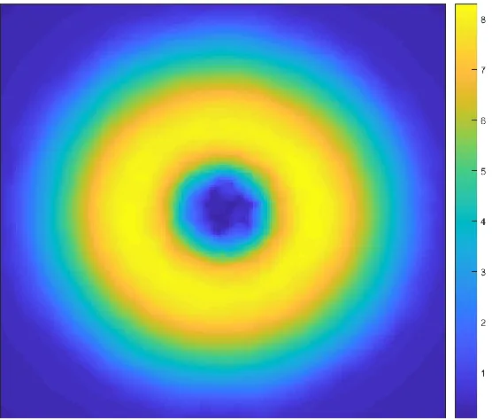
Figure 5.2 Thermal flux plotted using option 2 for the BeRP Ball in HDPE Shell ... 58
Figure 5.3 Fast flux plotted using option 3 for the BeRP Ball in HDPE Shell ... 59
Figure 5.4 BeRP Ball in Reflector Tessellated with SolidWorks ... 60
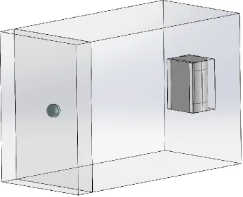
Figure 5.5 BeRP ball in cube of air rendered by SolidWorks ... 68
Figure 5.6 Adaptive Mesh of the SNAP Detector ... 75
Figure 6.1 Flux Due to a Point Source in a Vacuum at Cube’s Outer face ... 78
Figure 6.2 Flux at Cube’s Outer Face Due to BeRP Ball in Air with S2 Quadrature ... 79
Figure 6.3 Flux at Cube’s Outer Face Due to BeRP Ball in Air with S4 Quadrature ... 80
Figure 6.5 Flux at Cube’s Outer Face Due to BeRP Ball in Air with S16 Quadrature ... 81
Figure 6.6 S2 Coupled with MC Uncollided Flux at Cube’s Outer Face Due to BeRP Ball in Air ... 83
Figure 6.7 S2 Coupled with MC First Collided Flux at Cube’s Outer Face Due to BeRP Ball in Air ... 84
Figure 6.8 S2 Coupled with MC Second Collided Flux at Cube’s Outer Face Due to BeRP Ball in Air ... 85
Figure 6.9 S2 Coupled with MC Third Collided Flux at Cube’s Outer Face Due to BeRP Ball in Air ... 86
Figure 6.10 S2 Coupled with MC Fourth Collided Flux at Cube’s Outer Face Due to BeRP Ball in Air ... 87
Figure 6.11 Coupled Hammer-THOR Results and Reference Value for SNAP without the HDPE Shield ... 92
Figure 6.12 Coupled Hammer-THOR Results and Reference Value for SNAP with the HDPE Shield ... 94
Figure 6.13 Coupled vs Uncoupled SNAP Count Rates with and without HDPE Shield ... 95
Figure 7.1 Coupling Implementation Flowchart ... 98
Figure 7.2 Results Progression for the SNAP without the HDPE Shield ... 102
Chapter 1. Introduction
The problem of ray effects in transport calculations is important in nonproliferation and
radiation shielding problems. Since the propagation of a localized source cannot be accurately
calculated using discrete ordinates methods through low scattering media (such as air) ray effects
are common in configurations involving detectors separated from a localized source by air. As
such, efforts have been previously made to mitigate or eliminate ray effects in discrete ordinates
transport calculations.
Perhaps the most common method of mitigation involves the tracing of rays from points
used to approximate the localized source to computational cells where the flux is desired across
the low scattering media. The radiation is then propagated and attenuated along these rays and an
effective flux is rebuilt in the desired cells in order to compute a first collision source distributed
in each cell. This method, sometimes referred to as the analytic point-kernel approach to cover
its broader use in full transport solution codes, is used in several transport codes including the
Denovo code that is part of the ADVANTG package [1]. Such an approach suffers from a few
problems. Firstly, complex source geometries can require multi-point approximations which can
be inaccurate or expensive to create. Additionally, the method can require prohibitively large
numbers of rays for a complex/large region of importance to be traced to. The region of
importance must be determined by the user ahead of time, and the source must be approximated
automatically, or manually. Finally, such a method is semi-analytic in its approach to rebuilding
the distributed flux from point values, with expressions that are often ad hoc (that is the methods
are an engineering approximation and without explicit mathematically foundation).
Another approach is one that appears to be both intuitive and practical, and that is to
method allows for ray effect mitigation with minimal additional effort on the part of the user
preforming the calculations since the quadrature order is simply increased, assuming the
high-order quadratures are available in the subject transport code. However, the traditional level
symmetric angular quadrature sets have practical limitations on the order that they can be
extended to. Special quadrature sets are often required for problems with severe ray effects, the
making of which can be difficult. Additionally, even upon creation of such a quadrature set, the
calculation with increased number of discrete angles becomes significantly more expensive, and
the quadrature order that will significantly reduce the error from ray effects must be determined
on a problem by problem basis.
An equivalent form of the discrete ordinates equation has been created using spherical
harmonics equations to mitigate ray effects [2]. This method allows for a cheap calculation that
mitigates ray effects. However as spherical harmonics equations contain the reciprocal of the
total macroscopic cross section, this method can be unstable for regions with exceedingly thin
optical thickness (such as air).
An analytic first collision source was also shown to be effective and applied in the first
collision source codes GRTUNCL and GRTUNCL3D in two- and three-dimensional
configurations, respectively, that are in use with the DOORS code collection among others [3].
This method involves the use of the analytic solution for a purely absorbing system to calculate
uncollided flux at all distances from a distributed source. However, for complex sources and
configurations this calculation can be prohibitively expensive.
The final method covered here for the mitigation of ray effects is through the coupling of
Monte Carlo simulations to compute the first collision source. The previously cited Denovo
collision source calculation [4]. Such a method begins by running a Monte Carlo simulation for
uncollided flux. Once this flux is calculated throughout the system, it can be multiplied by
scattering cross sections per computational cell to create a first collision source distribution
throughout the domain to be used as the “external” source in a subsequent discrete ordinates
calculation. Such a method benefits simultaneously from the lack of ray effects in Monte Carlo
simulations of the uncollided flux, and the low computational costs of discrete ordinates methods
for the rest of the solution. Such a calculation does assume that the flux field resulting from the
source is dominated by uncollided particles on their way towards the region of importance (such
as inside a detector). This assumption is generally good since ray effects are a phenomenon
associated with materials with low collision rates.
It is a variation of this method that we adapt in our new mitigation strategy presented in
this work. We propose a mitigation method that uses Monte Carlo techniques to simulate an
arbitrary n–1 number of collisions and similarly uses the results from those collisions to compute
an nth collided source. This will enable the mitigation of ray effects to be more robust for systems where more than just the uncollided flux suffers heavily from ray effects.
The experiment used to verify our new method for mitigating ray effects and to validate
the THOR code consists of the weapons grade plutonium BeRP Ball on a stand sitting on a table
with detectors set up on the table. Previously, constructive solid geometry (CSG) models have
been made for both the ball itself as well as for the detectors that we used (MC15 and SNAP) in
a configuration suitable for modeling with MCNP.
The remainder of this thesis is organized as follows. In Chapter 2 we review previously
related work. Here we introduce transport theory and methods of solving neutron transport
established methods of mitigation. Finally, we examine previously performed experiments of the
same style as the ones performed for this work.
In Chapter 3 we examine the experimental setup performed for this work. This chapter
also investigates and draws conclusions from results measured in performing these experiments.
Chapter 4 introduces the MCNP models of the experiment that will serve as the basis of
our computational systems. This chapter examines both the full MCNP model and its results
created by Los Alamos, as well as the simplified MCNP model created for our computational
experiments. The errors introduced by each change in the process of creating this model are
quantified, recorded, and justified.
Chapter 5 discusses the development of the capabilities needed to perform our method of
ray effect mitigation. First, the chapter introduces four capabilities to be introduced to THOR in
order to enable easier problem computation and examination of results. This begins with
discussing verification of the manner of introducing subcritical multiplication to THOR. Then a
flux plotting method is discussed for use in visualizing computational results from THOR. This
is followed by discussion of the mesh generation method for THOR compatible meshes. Finally,
the method of converting SERPENT generated cross sections to THOR compatible data is
introduced. The chapter then introduces and derives the general collision Monte Carlo to SN
coupling method to mitigate ray effects and describes the implementation of the method. Finally,
the chapter introduces two different models to examine ray effects mitigation. The first features
an isolated source in a cube of air for visual examination of ray effects. The second is a detector
model described in Chapter 4 made in order to demonstrate the practical implications of ray
Chapter 6 presents and discusses computational results using both pure SN THOR
calculations as well as coupled calculations. The results here demonstrate the effectiveness of the
method in mitigating ray effects both visually and practically in nonproliferation applications.
Chapter 7 offers conclusions from results both experimental and computational in this
thesis. The method and model are also discussed, and the chapter includes discussion of the
numerical validation of this method and THOR for these types of problems. Finally, potential
Chapter 2. Review of Related Work 2.1 Neutron Transport Methods
2.1.1 Transport Theory and Equation
For systems where many neutral particles are interacting in a distributed physical space,
time, and velocity, certain statistical rules may be better suited to describe the behavior of the
system. The most common statistically-aggregated model used in neutron transport problems is
the Boltzmann equation. Four postulates must be adopted to cast this equation [5]. First the
particles being modeled must move freely most of the time and interact with each other only
during collision events where collisions of more than two bodies are considered rare. Second, the
average distance between collisions is much greater than the characteristic particle size. Third,
the collision time must be much less than the time between collisions. Fourth, gradients of
inhomogeneity in the system must be gradual for the particles being modeled compared to the
scale on which they collide.
For neutron transport problems in shielding and reactor systems, these postulates hold in
almost all circumstances. This leads to the applicability of the linearized Boltzmann equation in
these applications. The specific form of the Boltzmann equation that is used in these problems
can be derived through particle balance in a considered phase space. Such a balance derivation
yields what is commonly known as the neutron transport equation,
[1 𝑣
𝜕
𝜕𝑡+ Ω⃗⃗ ⋅ ∇ + Σ𝑡(𝑟 , 𝐸)] 𝜓(𝑟 , 𝐸, Ω⃗⃗ )
= ∫ 𝑑Ω⃗⃗ ′∫ 𝑑𝐸′ Σ(𝐸′→ 𝐸; Ω⃗⃗ ′ → Ω⃗⃗ , 𝑟 )𝜓(𝑟 , 𝐸′, Ω⃗⃗ ′) + 𝑆(𝑟 , 𝐸, Ω⃗⃗ )
2.1
where 𝜓(𝑟 , 𝐸, Ω⃗⃗ , 𝑡) is the neutron flux distribution and magnitude at location 𝑟 , comprised of
cross section and Σ(𝐸′→ 𝐸; Ω⃗⃗ ′→ Ω⃗⃗ , 𝑟 ) is the cross section for particles with energy 𝐸′ and angle
Ω
⃗⃗ ′ to produce particles of energy 𝐸 and angle Ω⃗⃗ . This integro-differential equation is a simplified
form of the full Boltzmann equation and is useful and suitable for work in neutron transport.
But this equation is complicated in nature and it provides analytic solutions in only a few
select cases that are generally highly simplified and not sufficient descriptors for the real-world
applications. This fact prompts numerical methods for obtaining approximate solutions in low- to
high-fidelity models of realistic applications. Methods for direct numerical solutions of this
equation often require discretization of the neutron energy spectrum [6]. Such discretization is
rooted in the fundamental concept that conservation of reaction rates in the system is essential
for a useful solution to the transport equations. This concept stems from the fact that the behavior
of a neutron system and most quantities of interest to nuclear scientists and engineers is driven
by neutron interactions with the host medium. From neutron streaming across regions, to reactor
power levels and associated local peaks of production through fission, to the interaction rate in a
detector providing a response, the conservation of reaction rates is essential to a useful solution
to the transport equation. As such the defined multigroup, or energy discretized, cross sections
optimally take such a form as to conserve corresponding reaction rates in Eq. 2.2 throughout all
regions of the domain,
Σx,g=
∫𝐸𝑔−1𝑑𝐸 Σ𝑥(𝐸)𝜙(𝐸)
𝐸𝑔
∫𝐸𝑔−1𝑑𝐸 𝜓(𝐸)
𝐸𝑔
2.2
where Σ𝑥(𝐸) is the cross section associated with interactions of type x. Definitions similar to Eq.
[1 𝑣𝑔
𝜕
𝜕𝑡+ Ω⃗⃗ ⋅ ∇ + Σ𝑡𝑔(𝑟 )] 𝜓𝑔(𝑟 , Ω⃗⃗ , 𝑡)
= ∫ 𝑑Ω⃗⃗ ′ ∑ Σ
g′→𝑔(Ω⃗⃗ ′→ Ω⃗⃗ , 𝑟 )𝜓𝑔′(𝑟 , Ω⃗⃗ ′, 𝑡) 𝑁𝑔
𝑔′=1
+ 𝑆𝑔(𝑟 , Ω⃗⃗ , 𝑡)
2.3
where Σ𝑡𝑔(𝑟 ) is the total cross section effective in group g and Σsg′→g(Ω⃗⃗
′→ Ω⃗⃗ , 𝑟 ) is the
production cross section in group g from incident neutrons in group g’. Many practical problems
in neutron transport are considered as steady state problems, causing the time derivative term to
vanish. For the remainder of this work, discussion of neutron transport will be considered
exclusively for steady state problems unless otherwise noted.
For complicated geometries there are a few methods of dealing with the angular
dependence of the neutron flux. One method is the discrete ordinates method, which solves the
solution along discrete rays that then influence other rays in the set via coupling in the
production term. This method will be expanded on later in the discussion.
Another common method of angular discretization is the expansion of the scattering cross
sections through Legendre polynomials and expansion of the flux in Spherical Harmonics.
Limiting the set of polynomials by truncating an angular derivative yields the spherical
harmonics equations, or the PN approximations [7]. This is often performed by truncating the
spherical harmonics equations at N=1 to give the P1 equations leading to Fick’s law. This in turn
gives the so-called neutron diffusion equation. This equation is commonly used in reactor
calculations as it is generally much cheaper and simpler to solve compared to the full transport
equation. However, no angular information is retained in diffusion theory for the flux, and this
can result in low accuracy in regions of highly anisotropic flux.
𝜓(𝑟 ∈ 𝜕𝑉, 𝐸, Ω⃗⃗ , 𝑡) = Γ(𝐸, Ω⃗⃗ , 𝑡) for 𝑛̂ ⋅ Ω⃗⃗ < 0 2.4
where 𝑛̂ is the outward normal vector of the bounding surface 𝜕𝑉 at the point r. These conditions
can take a variety of forms including reflective boundary conditions, vacuum boundary
conditions, and incident flux boundary conditions.
2.1.2 Monte Carlo Simulations
Solutions of the neutron transport equation can be obtained without solving the transport
equation. Perhaps the most common method involves direct simulation of particle histories
through Monte Carlo methods of sampling collision events based on the underlying neutron
physics [8].
The standard application of this technique involves randomly starting a simulation of a
particle history somewhere in the domain based upon a defined probabilistic physical distribution
of the source in the domain. For example, if the source is defined to be evenly distributed over a
sphere’s volume, the particle will be sampled somewhere in the sphere with all locations in the
sphere bearing an equal probability of being sampled. The particle is then sent in a random
starting direction based on the definition of the angular distribution of the source (often isotropic
for an external source).
The particle’s trajectory is traced along this starting direction with probability of
interaction in each region it moves through based upon the total cross section of the medium in
that region, which in turn gives the region a defined optical density. This optical density gives
the particle a chance to interact in a region or to move through an entire region without
interaction along its current trajectory, based upon pseudo-random number sampling. If the
particle is determined not to interact, it continues its current direction until either interacting in
the interaction occurs somewhere along the path in the region determined by a random sampling
based on the optical thickness. The type of interaction that occurs is also determined by a random
sampling based on the relative magnitude of the cross sections for different interaction types. If
the interaction produces new neutrons, through fission or scattering, the secondary neutrons are
now given a random direction from that point based on the angular distribution of the neutron
production (usually isotropic for fission but often anisotropic for scattering).
For an external source problem, all sampled particles are followed until they have been
eliminated fully by either exiting the domain or interacting in a manner that does not produce
secondary neutrons (absorption into a nucleus). This is done many times and the overall results
are interpreted to effectively give a solution to the neutron transport equation in the system with
related statistical error based on the number of particles started. Clearly this approach cannot be
expected to accurately predict the behavior of a single neutron as the probabilities do not
represent individual event physics. However, for many-particle simulations (as is required for the
Boltzmann equation to be valid), the behavior of the system can be well modeled by Monte
Carlo techniques.
Monte Carlo techniques have a few beneficial characteristics that methods for directly
solving neutron transport equation generally lack. First, they can utilize more accurate
geometries and do not require decomposition of physical geometry into cells. Objects are usually
defined using constructive solid geometry (CSG) which allows exact and human readable
expression of a geometry composed of combinations of geometric concepts, such as spheres,
cylinders, and planes. Additionally, Monte Carlo simulations depend on full probabilistic
distributions for neutron interactions, and therefore do not suffer the common deterministic
to provide a more complete model of the neutron flux energy spectrum compared to a
deterministic method. It is for this reason that a common method of multigroup cross section
generation involves the use of Monte Carlo solutions of simplified problems to produce spectra
at various energy cutoffs to preserve reaction rates in accordance with Eq. 2.2. These cross
sections from simplified problems can then be used in more complex, but similar, systems for the
faster deterministic methods to solve.
The biggest problem afflicting Monte Carlo techniques is the cost associated with the
simulation process. Because the uncertainty in the computed results is inversely proportional to
the number of particles sampled, complicated systems may require a prohibitively large number
of simulations to generate an adequately accurate result. There are a few ways to mitigate this
cost though. Firstly, since neutron systems are generally modeled for static environments, the
cross sections of regions are unchanging in the model regardless of neutron interactions. For this
reason, each particle can be treated independently without respect to other particles in the
system. Such independence opens many possibilities in the realm of parallel computations for
Monte Carlo simulations. Secondly, variance reduction techniques exist to reduce the uncertainty
in the simulation results without incurring a significant increase in the computational cost. These
techniques range from intuitive tactics such as factoring in path length in a regions flux tally, to
more complex concepts such as statistical weight reduction of particles instead of killing them
with absorption or system leakage.
2.1.3 Hammer
The Hammer code is one such Monte Carlo transport solver [9]. The Hammer code was
developed with the intention of supporting deterministic methods for solving neutron transport
Hammer code is different from many common Monte Carlo solvers in that it does currently rely
on multigroup cross section information. This improves the speed of the calculations, and the
ease with which the results may support deterministic codes, however it does mean that the
errors incurred by multigroup cross sections are present in Hammer results.
Hammer’s system geometry is based off of the standard method of CSG in 3D, however
it supports flux tallying on tetrahedral cells after the simulation has completed. The tallying is
done by mapping interaction collision points to the cells in which they occur. This tally is finally
compared to the number of particles started and divided by the total cross section of the cells to
determine a flux in the cell. This tallying allows for easy input into deterministic codes that break
up the problem domain into tetrahedral cells. Hammer also supports a number of variance
reduction techniques to improve the quality of flux estimation in regions of low interaction rate.
Perhaps the most important feature of Hammer’s capabilities for supporting deterministic
codes is the option to kill off particles after a certain number of collisions, and scoring all
interactions based on their collision count. Such tracking of collision count allows for an
accurate output of nth collided neutron flux throughout the problem domain. The method in which deterministic codes can be supported by Hammer requires flux of nth collided neutrons as well as all flux from lower collision-count neutrons. That is to say, the sum of all flux from
uncollided flux to nth collided flux. This is necessary to create a full description of the flux solution, as will be explained later, and this feature is supported in Hammer.
2.1.4 Discrete Ordinates
For deterministic methods of solving the transport equation the angular domain must be
discretized in order to permit numerical solution. One of the most common methods of achieving
method consists of solving the transport equation along a set of discrete angular directions [10].
In three-dimensional Cartesian geometry the discrete ordinates, or SN equations, are formulated
as Eq. 2.5 with the effective distributed source described by Eq. 2.6. These equations represent
the case of steady state multigroup neutron transport where all the secondary particles are
emitted isotropically, [𝜇𝑛 𝜕 𝜕𝑥+ 𝜂𝑛 𝜕 𝜕𝑦+ 𝜉𝑛 𝜕
𝜕𝑧+ Σ𝑡𝑔(𝑟 )] 𝜓𝑔(𝑟 , Ω⃗⃗ 𝑛) = 𝑄𝑔(𝑟 ) 2.5
𝑄𝑔(𝑟 ) =1
8 ∑ Σ𝑔′→𝑔(𝑟 ) ∑ 𝑤𝑛𝜓𝑔′(𝑟 , Ω⃗⃗ 𝑛)
𝑁(𝑁+2)
𝑛=1 𝑁𝑔
𝑔′=1
+ 𝑆𝑔(𝑟 ) 2.6
Here the discrete ordinates quadrature set is made up of unit vectors Ω⃗⃗ 𝑛 = 𝜇𝑛𝑖̂ + 𝜂𝑛𝑗̂ +
𝜉𝑛𝑘̂ so that 𝜇𝑛2+ 𝜂
𝑛2 + 𝜉𝑛2 = 1. The quadrature set also includes direction weights 𝑤𝑛 to allow for
accurate integration over the unit sphere using the quadrature set as indicated in the secondary
particles production term in Eq. 2.6. Level symmetric sets have historically been very common
in their use in discrete ordinates codes and many codes today have them as one of the common
options. As such much of the discussion here will focus on level symmetric sets. Such sets
provide N(N+2)/8 ordinates per octant and similarly N(N+2) directions across the entire unit
sphere by reflecting the discrete ordinates from the first octant into the other seven octants.
These quadrature sets generally have practical restrictions though. One of the most
common sets is the LQn set associated with the Legendre Polynomials. This set is useful in
producing level symmetric quadratures up to S20, however at S22 negative weights begin to
appear. As such the highest order set of this type used is generally the S16 set, however even this
set is rarely utilized as the large number of angles incurs a large and often prohibitive
In external source application, the discrete ordinates equations are iteratively solved using
a zero-flux initial guess. Such an initial guess means that each subsequent iterate of the discrete
ordinates equations can be interpreted as the flux of particles that have experienced up to one
more collision than the previous iteration, with the first iterate interpreted as the uncollided flux.
The physical interpretation of solving the discrete ordinates equations in this manner is
computing the uncollided flux with the transport equation solely from particles emitted by the
external source then traveling along the discrete ordinates in the spatial domain. The secondary
production from this flux is then calculated in each cell using the cell’s effective secondary
production cross section. This leads to secondary production in the cell along all discrete
directions based on the angular distribution of the production. This leads to regions in which the
secondary production is high to tend to have secondary sources that are better distributed along
directions in that region compared to regions where the secondary production is low.
If the flux is dominated by neutrons that have experienced only a few scattering events
emitted from a localized source, then there exists a risk that the flux will not be well distributed
along all directions in regions far from the localized source. This risk comes from the fact that
only directions that trace back directly to the source will see the uncollided flux. As such, if the
uncollided flux is dominant, the secondary production will in turn be low, resulting in flux
focused along the rays that “see” the source. This results in the numerical artifacts known as ray
effects and can be one of the biggest errors incurred in a discrete ordinates calculation. These
artifacts prompt much of the work presented in this thesis and will be discussed at length later.
Discrete ordinates methods tend to be some of the fastest and most efficient methods for
solving neutron transport problems. They retain angular flux information, unlike the diffusion
projections onto Legendre Polynomials. As the angular fluxes along different angles are
mutually independent in each sweep assuming Cartesian geometry and explicit boundary
conditions, the potential for high degrees of parallel processing exists. There are also several
iterative acceleration techniques that can be applied to solving the transport equation with the
discrete ordinates approximation. Many of these are dependent on efficiently solving some form
or variation on the spherical harmonics equations to estimate what the final flux should look like.
All this leads to discrete ordinates methods often being seen as a good middle ground in terms of
computational efficiency, easily beating the speed of continuous energy Monte Carlo but often
slower than diffusion solutions, and solution accuracy, better describing angular flux effects than
diffusion but maintaining errors of energy, space, and angle discretization’s that are not incurred
in Monte Carlo simulations. Instead, the latter incurs quantifiable statistical errors.
2.1.5 THOR
The THOR (Tetrahedral High-Order Radiation) transport code is a steady-state,
multigroup, discrete ordinates transport solver for 3D, unstructured tetrahedral meshes [11].
THOR is currently maintained by the Consortium for Nonproliferation Enabling Capabilities
(CNEC) and draws its origin from Dr. Rodolfo Ferrer’s dissertation at Pennsylvania State
University [12]. THOR solves the discrete ordinates equations on tetrahedral cells using the
method of short characteristics where spatial moments of the flux are solved along characteristics
traversing a cell, thus providing boundary conditions for the cell to interface with the flux in
neighboring cells. The within-cell angular flux moments also enable evaluation of angular
moments that facilitate the computation of the distributed source of secondary particles in an
THOR supports eigenvalue solutions for supercritical, subcritical, and critical systems as
well as external source solutions for non-multiplying and subcritical systems. THOR supports
both isotropic and anisotropic scattering and has a variety of built-in angular quadrature sets.
Recent applications of THOR include nonproliferation scenarios to solve complicated
three-dimensional configurations involving source detection, shielding, and criticality.
As a discrete ordinates code, THOR suffers from errors introduced by energy and angular
discretization. Additionally, spatial errors are present due to using cell moments of the flux to
determine secondary production density-rates as well as the inability of tetrahedrons to fully
describe curved geometries. But, with good cross sections and a well resolved unstructured
mesh, these errors are often acceptable. A bigger concern for THOR in shielding and
nonproliferation applications is ray effects.
As a transport code, THOR is an effective application of high order discrete ordinates
equations and can provide fast three-dimensional solutions with highly efficient parallel
capabilities. As such its use in three-dimensional nonproliferation applications remains of great
interest to CNEC. This then prompts efforts to mitigate ray effects for the THOR code to enable
more accurate and realistic neutron transport solutions in those applications.
2.2 Ray Effects
2.2.1 Description of Effects
Discrete ordinates methods solve the radiation transport equation along discrete angles in
phase space. If the in-group scattering term is sufficiently large, the source due to collisions of
the transported particles, or secondary source, is well distributed throughout the problem
geometry. However, in low in-group scattering media the secondary source does not illuminate
propagation only along angles that directly trace back to the localized source. Such “ray effects”
can result in non-physical flux profiles that exhibit low illumination of cells not along the rays
that reach back to the source, as well as over estimation of the flux along the rays.
Anomalous calculation results were first observed in 1965 from discrete ordinates
approximations to the two-dimensional Boltzmann transport equation [13]. At about the same
time similar inconsistencies in 2-D SN calculations were noticed. It was gradually realized that
the anomalies were not numerical truncations errors but due to the discrete ordinates formulation.
With a limited number of discrete angles, there are a limited number of directions along which
streaming can occur. So, neutron flux contributions in a region far from a localized source are
limited to locations where angular directions in the quadrature set can be traced back directly to
the localized source.
Though 2-D SN computations have been practiced since 1959, these “ray effects” were
not recognized in discrete ordinates until 1965 and it was theorized that this may be because the
discrete ordinates formalism was derived by heuristic arguments for finite phase space cells [13].
The nature of these ray effects in the discrete ordinates approximations have been examined. It
was pointed out that the severity of the ray effects is dependent upon the nature of the sources.
Highly localized sources provide harsher ray effects as they result in more "dead zones" with
respect to streaming characteristics. An example is shown in Fig 2.1 copied from [13], where the
medium is a pure absorber, so the source is only present in the rectangular area on the right side
Figure 2.1: Monoenergetic Ray Effects in Discrete Ordinates Solution.
The problem shown featured a highly localized source. The characteristic directions from
the source corners are shown in the figure, resulting in a dead zone on the far-left boundary
where none of the characteristic curves both intersect the source on the far right, and the
observation point on the far left. This results in all characteristic curves streaming into this
triangular dead zone to be streaming zero source from a discrete ordinates perspective. This is
clearly seen to be wrong as in the real world the dead zone points would experience a flux that is
not only similar, but assuming the source is uniformly distributed in its region, but even larger
than at the corners, which are seen to experience a positive flux. It should be noted here that ray
effects are a geometric phenomenon therefore energy discretization is irrelevant to the
demonstration of these effects.
A more complex case that was examined in [13] was the situation of four local fuel
elements present in an absorbing material. An unexpected case of higher top flux than bottom
flux was observed in the S2 calculation, which was then mitigated by the higher order S4
calculations. However, both showed an unexpected peak in the absorbing channel. It was
conjectured that this may be due to lower absorbing properties of the channel. But it was
the four different sources along the 45o angle, which is present in all SN orders and angular sets. This local maximum at the channels was determined to be a subtler ray effect than that on the
boundary but present for all orders of discrete ordinates equations.
The potential problems with ray effects in shielding and detector problems for SN
methods is immediately apparent. For a detector a distance away from a localized source, the
rays may cause one of two issues. The first potential issue is that no rays may intersect both the
local source and the local detector. The primary rays along the source missing the detector in this
way would result in a count rate far below the physical expectation if the region between the
source and the detector is composed of a low scattering material. This is because practically no
particles will be transported from the source to the detector in this calculation.
Alternatively, the opposite, yet no less concerning, error is also possible. Since the
discrete ordinates equations have no explicit term for geometric attenuation, the flux along the
rays that intersect the source is subject to only material attenuation when compared to the source
strength. Since ray effects are most common in low interacting regions, and low scattering
regions tend to also have low total interaction rates, the flux along the ray ends up being
significantly large compared to the physically expected value. Such large flux rays intersecting
with a detector could result in significantly higher count rates in the detector than physically
expected.
In the end, the best-case scenario for a problem with ray effects would be the cancellation
of errors. Having offsetting number of peaks and troughs of interaction from the source along the
rays going through low scattering regions. However, such a case is made increasingly unlikely as
the region affected by ray effects becomes larger and the detector goes further from the localized
It therefore becomes clear that nonproliferation and shielding problems are perhaps the
most affected by ray effects. Most such problems have large regions of air separating a very
localized radiation source from a target model or point detector. Propagation through air with
discrete ordinates equations results in massive ray effects as the secondary source production
diminishes due to low optical thickness of air. As a result, dose or detector count rate estimates
are often inaccurate when computed using just discrete ordinates methods, unless one is lucky
enough that a cancellation of errors occurs.
However, the impact of ray effects reaches beyond just nonproliferation and shielding
problems. While it is often assumed that ray effects are small or negligible in a large-scale
reactor, due to fission sources that are often well distributed and the presence of highly scattering
materials, studies have shown that ray effects can be a significant issue in fast reactor simulations
[14]. Indeed, design studies of fast reactors with local heterogeneities, such as non-fuel control
rods or instrument channels, have shown that power distributions in such designs are badly
distorted when computed by low-order discrete ordinates quadratures. This error appears to be
severe enough to raise concerns that thermal-hydraulic calculations using results from such
equations may result in improper distribution of coolant flow and local overheating. So, while
this work may primarily concern itself with ray effects and their mitigation for the purpose of
nonproliferation applications, it should be kept in mind that ray effects, and by extension the
need for their mitigation, appear in a variety of nuclear applications.
2.2.2 Mitigation Through Special Quadrature Sets
The most direct method of ray effect mitigation is through increasing the number of
angles comprising the SN quadrature set employed in the calculation. While ray effects must still
troughs will intersect a given location of interest, such as a detector, is drastically increased by
having the location closer to the source, and by increasing the number of discrete directions to
solve along. Such increase in spatial directions has been investigated [15]. Results showed that
S2 calculations provide a substantially less accurate solution in cases where severe ray effects are
observed compared to S16. However, it was illustrated that even with this remedy there are still
ray effects contaminating the solution and they can exhibit defects requiring even higher order
angular quadratures, which is not a practical remedy in terms of computational costs. A problem
with a square source centrally located source in a square domain with 𝑐 =Σ𝑠
Σ𝑡 = 2/3 was solved
in [15] and yielded results that demonstrated severe ray effects. Even with a S16 (144 directions)
solution the ray effects are still quite visible, and this in a problem where the source covers an
entire quarter of the domain and the scattering is nonzero. The fact that 144 directions is not
sufficient to eliminate the distortion of the flux at the domain’s edge suggests that simply
increasing the number of discrete ordinates is unlikely to be yield a satisfactory solution to the
problem of ray effects in a general setting. This is especially true in detector problems where
sources tend to be physically small in comparison to the entire domain size.
Alternatively, special quadrature sets have been proposed and examined [15]. These
quadrature sets are usually specific to a given problem, not generally applicable. One example
involves arranging directions to preserve rotational invariance properties of the divergence
operator. Results of numerical tests for the same square-in-square configuration described above
using these sets (called RN sets) were examined in [15].The distortions are reduced better than
with the standard level symmetric quadrature sets originally used to show ray effects, however
even with the expensive R16 set, visible ray effects persisted. The examined specialized sets
improvement is not significantly sufficient to avoid extremely high-order sets in more extreme
cases.
In any case, it seems unlikely that special quadrature sets can provide a sufficient and
general solution to ray effects that afflict discrete ordinates methods. Additionally, while
increasing the order of the discrete ordinates quadrature set does show reduction in ray effects in
general, such a method may require prohibitively large number of angles to solve problems of
large physical extent suffering from severe ray effects.
2.2.3 Mitigation Through Spherical Harmonics Equivalence
Not relying on a collocation approach to angular discretization, the projection-based
spherical harmonics method is immune to ray effects. This property has motivated the creation of
discrete ordinates equations that are equivalent to the spherical harmonics equations. This
method was implemented for the abovementioned square-in-square test problem [13]. The flux
profile associated with the modified S2 equations suffered from no ray effects, while the standard
S2 solution had clearly visible ray effects. The flux profile for the spherical harmonics equivalent
solution matched exactly with a spherical harmonics solution of the problem.
A variation on this approach uses an interpolation method to formulate a proper fictitious
source and boundary conditions for the problem to make it equivalent to the spherical harmonics
[2]. This method results in a consistently high order method in the transformation between the
discrete ordinates equations and the spherical harmonics equations, i.e. SN PN equivalency. In
fact, a general method of transformation to make any SN set of equations equivalent to PN
equations has been demonstrated [2]. Such a method shows that for any discrete ordinates order,
The fictitious source method has been one of the most studied methods for spherical
harmonics equivalence [16]. These sources seek not to attempt an entire transformation of the
discrete ordinates equations to achieve equivalence with the spherical harmonics equations,
rather they introduce a derived fictitious source term that will enforce the equivalency. The goal
of such methods is to create situations were standard methods of solving the discrete ordinates
equations can still be utilized but with the added source term to give spherical harmonics
qualities to the solution. However, it must be recognized that derivation of the spherical
harmonics equivalent source is non-trivial and unique for each quadrature order of discrete
ordinates equations. Composing the source involves expanding the scattering cross section,
angular flux, and external source using spherical harmonics, then inserting these newly expanded
terms to the transport equation and applying the recursion formulas for the spherical harmonics.
Comparison between this resulting equation and the SN equations yields a fictitious source to
give equivalence.
While this method does seem promising for application in trouble regions to eliminate
ray effects, there is a concern arising from its equivalence to the spherical harmonics equations
that normally include the reciprocal of the host material total cross sections. This division may be
acceptable to resolve ray effects in highly absorbing media where the total cross section is
reasonably large but the scattering ratio is small. However, for configurations common in
detector and nonproliferation applications, which often include air, both total and scattering cross
sections are very small so that division by the former may cause instability in the solution. Such
2.2.4 Mitigation Through Semi-Analytic Method
Mitigation of ray effects is possible through a more analytic approach. The GRTUNCL
code was created for use with the two-dimensional transport code DORT and showed practical
application of an analytic method for mitigating ray effects [17]. GRTUNCL solves for an
uncollided flux throughout the domain analytically and is then transformed through ad hoc
methods to create cell averaged scalar flux, which then in turn provides a first collision source to
the DORT code. The computational method employed for this approach begins with
𝜙𝑢,𝑔(𝑟 𝑖) = ∑ 𝑆𝑔(𝑟 𝑘)𝑒−𝛽𝑔(𝑟 𝑘,𝑟 𝑖)
Δ𝐴𝑘
4𝜋|𝑟 𝑖− 𝑟 𝑘|2 𝑘
2.7
Here 𝜙𝑢,𝑔(𝑟𝑖) is the uncollided scalar flux in energy group g at location 𝑟 𝑖 due to an
isotropic distributed source spanned by the discretized points 𝑟 𝑘. 𝑆𝑔(𝑟 𝑘) is the number of source
particles emitted per unit time at point 𝑟 𝑘 across the area associated with that source disk Δ𝐴𝑘.
𝛽𝑔(𝑟 𝑘, 𝑟 𝑖) is the number of mean free paths along the vector from 𝑟 𝑖 to 𝑟 𝑘. Evaluating this
equation gives an estimate of the uncollided scalar flux at point 𝑟 𝑖, where the primary error
incurred is the approximation of a distributed source by a set of point sources. The result is then
plugged calculated for Eq 2.8 to provide a first collision source for the computational cell
centered at ri
𝑆𝑔(𝑟 𝑖, Ω⃗⃗ ) = ∑ ∑𝐴
𝑙,𝑚(Ω⃗⃗ )
4𝜋 ∑ Σ𝑔′→𝑔 𝑙 (𝑟
𝑖) ∑ 𝑆𝑔(𝑟 𝑘)𝑒−𝛽𝑔(𝑟 𝑘,𝑟 𝑖)
𝐴𝑙,𝑚(Ω⃗⃗ 𝑘)Δ𝐴𝑘
4𝜋|𝑟 𝑖− 𝑟 𝑘|2 𝑘
𝑔′ 𝑚
𝑙
2.8
This is now a space, angle, and energy dependent first collision source derived from Eq.
2.7 representing the uncollided flux. Here Ω⃗⃗ 𝑘 represents the unit vector from 𝑟 𝑖 to 𝑟 𝑘, 𝐴𝑙,𝑚(Ω⃗⃗ ) are
in the Legendre expansions of energy group-to-group scattering cross sections. All this together
provides an analytic estimate of first collision source from a set of point sources.
The procedure of implementation goes as follows. First the geometry is described with
the same spatial mesh used for the DORT problem. Next the uncollided flux is calculated for
each selected spatial point and energy group. Then the first collision source is calculated for each
point, energy and angular moment and written to an output file. Finally, the first collision source
is used as DORT input in the form of an anisotropic fixed source array. DORT can then calculate
the fully collided flux angular moments and combine them with the uncollided flux moments
produced by GRTUNCL to get the total flux in the system.
This method was implemented and developed specifically for two-dimensional r-z
geometry to go along with the transport code DORT, however there is no reason such a method
could not be applicable in any geometric system. In fact, the method has been expanded to full
3D application in x-y-z geometry [18] and later r-θ-z geometry to compute first collision source
moments [19]. Specifically, the r-θ-z application was used to mitigate ray effects in the TORT
three-dimensional discrete ordinates computer code. The method was applied to the problem
geometry composed of a cylinder of air containing a semicircular wall shielding a source.
This problem involved a gamma ray point source in the center of a semicircle concrete
shield. The height of the source was 20m from the surface of the ground, or halfway up the 40m
shield. The results of the calculation without GRTUNCL3D first collision source showed severe
ray effects for the pure TORT calculation. Then combination with GRTUNCL3D demonstrated
major mitigation of the ray effects in the air. The use of GRTUNCL3D was also demonstrated in
eliminating most primary ray effects using GRTUNCL3D and demonstrated the practical
application of the method.
This method is not without limitations though as its computational cost becomes
prohibitive for general problems. For an arbitrary source distribution discretized into a set of
point sources, rk, the contribution from each point source must be computed thus conferring a
computational cost that is directly proportional to the number of point sources, per Eq 2.8.
Additionally, complex geometries and fine meshes may require many field points, ri, for first
collision sources to be calculated at. This all can mean that for complicated meshes and source
distributions, the costs associated with implementing a semi-analytic solution can be prohibitive.
This method is generally effective and efficient in simple geometries with simple source
distributions. However even in such situations the method is still limited by its inability to
estimate sources of higher collision orders than first. As such, in problems where severe ray
effects are prominent in higher collided flux and higher collided particles dominate the flux
distribution, one can expect little mitigation through application of the analytic first collision
source method.
2.2.5 Mitigation Through Point-Kernel Method
The point-kernel method for radiation transport is a simplified method for considering a
point source propagation through a medium [21]. As shown in Fig 2.2, the flux is attenuated
along the rays drawn from the point source with attenuation dependent upon distances traveled
Figure 2.2: Point-Kernel Method.
The rebuilding of the flux is then done for the target cells that the ray is traced to. Such
rebuilding is ad hoc with methods that are dependent upon cell shapes, location in the cell the
lines are drawn to, and cell optical thicknesses.
For a problem using the point-kernel method to mitigate ray effects, the most common
method is to ignore scattered radiation buildup, a reasonable assumption in our target
applications since the problem area likely has a very low scattering rate. This now makes the
calculated flux the uncollided flux, able to become the first collision source in a like manner to
the analytic method. Once the uncollided flux is traced and attenuated to the cells it must be
rebuilt into cell averaged scalar flux. The rebuilt flux is then multiplied by the scattering cross
sections to create a first collision source, which is used to solve the rest of the problem using
discrete ordinates method [22].
Such a method may require tracing many rays in order to achieve acceptable accuracy.
The total number of rays is equal to the number of cells to be traced to multiplied by the number
of discretized point sources multiplied by the number of rays needed for each cell. This results in
multiple point source approximations and the geometry has many cells requiring tracing along
several rays each. Additionally, in a similar manner to the semi-analytic method, this method
cannot naturally estimate a collision source of higher collision-count than first.
2.2.6 Mitigation Through Monte Carlo Coupling
In problems where ray effects are severe, such as localized source problems, the transport
method of choice is often Monte Carlo since it does not suffer from ray effects. However, in
regions of many scattering collisions Monte Carlo simulations become expensive as it must
follow the particles to termination. A combination of Monte Carlo with SN methods has been
proposed where the first collision source simulated by a Monte Carlo code is fed into a discrete
ordinates code in a similar manner to the point-kernel or analytic first collision source methods
[23].
The method presented in [23] involves the usage of a Monte Carlo simulation, either
multigroup or continuous energy, to create a first collision source for a discrete ordinates
calculation to use as an “external” source. Like the semi analytic and point-kernel methods, this
method involves splitting the problem based on particles’ collision-count rather than by
geometric or energy boundaries. Now though, the method for determining the uncollided flux is
Monte Carlo rather than analytic or by ray tracing.
A problem is considered in [23] that is collision dominated, making it a prime candidate
for discrete ordinates solutions, but containing important regions prone to severe ray effects.
Such a problem would be expensive for a Monte Carlo simulation as the dominance of collisions
may require tracking the particles through many scattering events before they are terminated.
However, the low scattering material present in portions of the problem may cause catastrophic
could be a localized source in a room filled with air and a detector placed a distance away. The
detector is collision dominated and would require many collisions to fully resolve in a Monte
Carlo simulation, however the air separating the two would incur major ray effects in the
transport process from the localized source to the detector. This motivates using Monte Carlo to
calculate the first collision source and discrete ordinates to calculate the collided flux.
The method can be described through a derivation beginning with the original transport
problem in Eq. 2.1. The flux is rewritten as
𝜓(𝑟 , 𝐸, Ω⃗⃗ , 𝑡) = 𝜓𝑢(𝑟 , 𝐸, Ω⃗⃗ , 𝑡) + 𝜓𝑐(𝑟 , 𝐸, Ω⃗⃗ , 𝑡) 2.9
where 𝜓𝑢 is the uncollided flux and 𝜓𝑐 is the collided flux, then these fluxes satisfy,
1 𝑣
𝜕𝜓𝑢
𝜕𝑡 + Ω⃗⃗ ⋅ ∇𝜓𝑢(𝑟 , 𝐸, Ω⃗⃗ , 𝑡) + Σ𝑡(𝑟 , 𝐸)𝜓𝑢(𝑟 , 𝐸, Ω⃗⃗ , 𝑡) = 𝑄(𝑟 , 𝐸, Ω⃗⃗ , 𝑡) 2.10
1 𝑣 𝜕𝜓 𝜕𝑡 + Ω⃗⃗ ⋅ ∇𝜓𝑐(𝑟 , 𝐸, Ω⃗⃗ , 𝑡) + Σ𝑡(𝑟 , 𝐸)𝜓𝑐(𝑟 , 𝐸, Ω⃗⃗ , 𝑡) = ∫ ∫ Σ𝑠(𝑟 , Ω⃗⃗ ′ → Ω⃗⃗ , 𝐸′→ 𝐸)𝜓𝑐(𝑟 , 𝐸′, Ω⃗⃗ ′, 𝑡)𝑑Ω⃗⃗ ′𝑑𝐸′ 4𝜋 ∞ 0 + 𝑄𝑢(𝑟 , 𝐸, Ω⃗⃗ , 𝑡) 2.11
respectively, where 𝑄𝑢(𝑟 , 𝐸, Ω⃗⃗ , 𝑡) = ∫ ∫ Σ4𝜋 𝑠(𝑟 , Ω⃗⃗ ′→ Ω⃗⃗ , 𝐸′ → 𝐸)𝜓𝑢(𝑟 , 𝐸′, Ω⃗⃗ ′, 𝑡)𝑑Ω⃗⃗ ′𝑑𝐸′ ∞
0 and is
referred to here as the first collision source. Equation 2.9 satisfies Eq 2.1 under conditions 2.10
and 2.11. Therefore, this provides a method of coupling the first collision source to the fully
collided solution. Boundary conditions take the general form shown in Eq. 2.4. This makes the
boundary condition for the new, coupled pair of problems,
𝜓𝑢(𝑟 ∈ 𝜕𝑉, 𝐸, Ω⃗⃗ , 𝑡) = Γ(𝐸, Ω⃗⃗ , 𝑡) for 𝑛̂ ⋅ Ω⃗⃗ < 0 2.12
𝜓𝑐(𝑟 ∈ 𝜕𝑉, 𝐸, Ω⃗⃗ , 𝑡) = 0 for 𝑛̂ ⋅ Ω⃗⃗ < 0 2.13
so that all incoming flux into the problem is assigned to the uncollided flux portion, and the
for an original problem with explicit boundary conditions. Implicit boundary conditions, e.g.
reflective, would replace the right-hand sides of these equations with an expression involving 𝜓𝑢
and 𝜓𝑐, respectively.
It is worth noting that Eq 2.10 has the form of a purely absorbing medium with a fixed
distributed source and boundary conditions, therefore it can be solved analytically for simple
geometries and sources. But for the general case it can be solved efficiently via a Monte Carlo
simulation where a particle’s history is terminated upon its first collision. Equation 2.11 can then
be solved by the method of discrete ordinates using the solution from Eq 2.10 to build the first
collision source. Such a solution would eliminate ray effects in the uncollided flux and facilitate
calculation of the collided flux that is hopefully well distributed in collision dominated regions to
be solved in a computationally efficient manner.
However, for a geometry that results in a localized first collision source, e.g. a shielded
point source surrounded by air, ray effects may still afflict the collided flux in regions dominated
by higher collided flux. This is because the first collision source will be heavily concentrated in
the shield around the point source. In other words, severe ray effects are likely in the solution of
Eq 2.11 as it is used to model neutron transport across the low scattering regions propagating
from a first collision source localized in the source shield.
It is concluded that the method is conceptually simple and is best suited to a localized
source problem with regions that are collision dominated. However even in such problems,
secondary ray effects may still be a major concern in cases where the first collision source
remains localized.
This method was tested using MCNP for the Monte Carlo simulation and TWODANT