Drake, Kimberly J. Analysis of Numerical Methods for Fault Detection and Model Identi-fication in Linear Systems with Delays. (Under the direction of Steve Campbell.)
Recently an approach for multi-model identification and failure detection in the presence of bounded energy noise over finite time intervals has been introduced. This approach involved offline computation of an auxiliary signal and online application of a hyperplane test.
This approach has several advantages; but, as presented, observation over the full time interval was required before a decision could be made. We develop an algorithm which modifies this approach to permit early decision making with the hyperplane test.
SYSTEMS WITH DELAYS
by
Kimberly J. Drake
a dissertation submitted to the graduate faculty of north carolina state university
in partial fulfillment of the requirements for the degree of
doctor of philosophy
applied mathematics
raleigh, north carolina August 22, 2003
approved by:
Dr. Stephen Campbell Dr. Pierre Gremaud
chair of advisory committee
One day when you were a very, very little girl, you put on the apron and vest from my waitressing uniform and you played at taking orders from everyone in the house, including your dolls. You were so sweet, sassy and small, going from person to doll with equal gravity, taking orders in a language the rest of the family was too old to remember. As I watched you, I realized that you were not just playing at being a waitress; you were playing at being me. I realized that day how very important it is that I be a woman who you could become. You are my inspiration.
Always remember that nothing is beyond your reach.
Kimberly J. Drake was born in Dover, NJ on January 7, 1970. She grew up in the small town of Budd Lake, NJ and graduated in 1988 from Mt. Olive High School. She worked her way through college, graduating from Montclair State University in 1996 with a B.S. in mathematics and computer science, as well as a teaching certificate.
After college, she moved briefly to Livermore, CA where she interned at the Lawrence Livermore National Laboratory. Leaving sunny California behind, Kimberly moved to Raleigh, NC where she attended graduate school at North Carolina State University, work-ing with Steve Campbell.
Her graduate school years included a time working at the Boeing Company with John Betts in Bellevue, WA and a time working at INRIA-Rocquencourt with Ramine Nikoukhah in Le Chesnay Cedex, France. After graduating with her Ph.D. in Applied Math, she plans to move to Philadelphia, PA to work for the Navy.
First, I would offer my gratitude to my advisor, Dr. Stephen L. Campbell. In addition to being a brilliant and successful scholar, he is also a patient and generous mentor.
I am grateful to the members of my committee: Dr. Pierre Gremaud, Dr. Ralph Smith, and Dr. Hien Tran. I am grateful to them for ensuring the quality of my work as well as for being excellent teachers. I would offer a special thanks to Dr. Gremaud who so cheerfully gave me many hours of his time through four courses and the qualifying exams, preparing me to do this work.
I would also like to thank Dr. John Betts and The Boeing Company, as well as Dr. Ramine Nikoukhah and INRIA-Rocquencourt. My time working with these men at their respective institutions was invaluable to my education and a true pleasure.
I also offer my thanks to the National Science Foundation, which supported this work. I would like to thank Dr. Leona Harris-Clark and Dr. Doug Cochran. The support of close friends is invaluable.
I am grateful to my family for their patience and understanding.
Finally, I would like to thank God. Without Him, none of this would have been possible.
List of Figures vi
1 Introduction and Background 1
1.1 Mathematical Background . . . 2
1.1.1 Optimal Control . . . 2
1.1.2 Solving the Optimal Control Problem . . . 4
1.1.3 Approximation Theory . . . 6
1.2 FDMI: Introduction and Prior Research . . . 7
1.2.1 Other Prior Research . . . 8
1.3 Fault Detection via the Minimum Energy Detection Signal . . . 10
1.3.1 Minimum Energy Detection Signal . . . 11
1.3.2 Model Identification by the Separating Hyperplane . . . 20
1.4 Outline of Thesis . . . 24
1.5 Contributions of Thesis . . . 24
2 Early Detection 26 2.1 What is Early Detection and Why Bother? . . . 26
2.2 Analytical Breakdown of Problem . . . 27
2.3 Algorithm . . . 31
2.4 Computational Tests . . . 36
3 True Solutions: The Method of Steps 39 3.1 Introduction to the Problem . . . 39
3.2 True Solutions with the Method of Steps . . . 42
3.2.1 The Basic Problem . . . 42
3.2.2 Necessary Conditions of the Optimal Control Problem and Proof of Optimality . . . 47
3.2.3 Minimum Energy Detection Signal Algorithm for the Method of Steps 54 3.2.4 Problem Variations . . . 55
4.2 Explanation of the Central Differences Approximation . . . 63
4.3 Necessary Conditions for the Fault Detection Problem . . . 65
5 Approximated Solutions: Spline Approximations 69 5.1 Explanation of the Spline Approximation . . . 69
5.2 The Optimal Control Problem Using Splines . . . 76
5.3 Theoretical Results . . . 78
5.3.1 Review of Familiar Theorems and Definitions . . . 79
5.3.2 Some Useful Lemmas . . . 81
5.3.3 How Close Are the Real and Approximated Output Sets? . . . 88
5.3.4 A Hyperplane Which Separates the Real Sets Separates the Approx-imated Sets . . . 90
5.3.5 A Hyperplane Which Separates the Approximated Sets Separates the Real Sets . . . 97
6 Examples and Analysis 101 6.1 Steps, Differences and Splines on a Single Delay . . . 102
6.2 Splines and Differences on Multiple Delays . . . 104
6.3 Splines and Differences on Mixed and Multiple Delays . . . 105
6.4 Mach Number in a Wind Tunnel . . . 106
6.5 Conclusions about Numerical Examples . . . 108
7 Future Work and Conclusions 109 7.1 Future Work . . . 109
7.2 Conclusions . . . 112
A Software 115 A.1 M-files . . . 115
A.2 Method of Steps . . . 115
A.2.1 Matlab Driver for the Method of Steps . . . 115
A.2.2 Method of Steps Driver . . . 122
A.3 Splines . . . 141
A.3.1 Matlab Spline Driver . . . 141
A.3.2 Spline Driver . . . 151
A.4 Differences . . . 162
A.4.1 Matlab to Generate System Matrices . . . 162
A.4.2 Differences Driver . . . 170
List of References 184
1.1 The figure illustrates a proper detection signal, v, pushing the output sets,
Ai(v), apart. . . 13 1.2 Using the hyperplane, a test can be formulated that will determine if y lies
above the plane or below it, determining from which model the output is produced. . . 21
2.1 An example of ψi,j . . . 28 2.2 Whenψi,j, the value of the hyperplane test which is calculated as the output
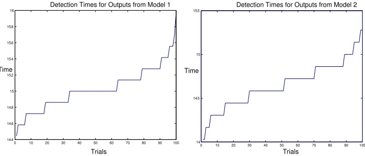
y becomes available, crosses δbi,j or −bδi,j, the test is complete. In 100 trials on each model, detection takes place around .75ω. . . 37 2.3 Detection time distribution for 100 trials of each model. The figures show
that over 60% of the trials had resulted in detection by t = 15, which is a reduction of 25% . . . 38
3.1 Diagram illustrating the Method of Steps: A new variable is assigned to each interval of length h of the detection horizon, where h is the length of the delay. Then variable zi−1 is the past history of variable zi and the system can be reformulated without the delay term. Using these new variables, a system of equations is set up, allowing the solution for the entire detection horizon to be found simultaneously. A boundary condition zi−1(h) =zi(0) is included to ensure continuity between variables. . . 44
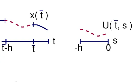
4.1 We reformulate the delayed system into a PDE by lettingU(t, s) =x(t+s) for 0≤t≤ω,−h≤s≤0. In the figure, U(¯t, s) is x(¯t). The dashed section of the curve represents U(¯t, s) for −h ≤ s≤ 0; that is, U(¯t, s) and its past history. . . 62 4.2 Having reformulated the problem into a PDE, we now use the method of
lines and central differences to approximate the PDE with an ODE. We first define a mesh −h=s0 < s1 <· · ·sρ= 0, where each delay must be a mesh point. Then we let Uk(t) = U(t, sk). This illustration represents the new variables when t= 0. Notice that the new variables will represent the past history needed because of the restriction that each delay must be a mesh point. . . 64
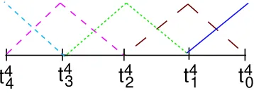
tNk travels backward in time. Notice also thattN0 = 0 and tNN =−r wherer
is the length of the longest delay. Thus, the spline functions are defined on an interval the size of the longest delay. . . 72 5.2 If a hyperplane separates the real output sets, then it also separates the
approximated output sets. More specifically, we show that given < y, a >≥ where a is a hyperplane, then for any δ > 0, there exists N such that if
n > N then for allyN ∈ ANi (v), < yN, a >≥ −δ. . . 91 6.1 The figure shows the Method of Steps, the spline approximation and the
difference approximation on the models (7.4) which have a single delay. A mesh size of 20 is used in each approximation. . . 102 6.2 The figure compares the Method of Steps and the spline and difference
ap-proximations on example (7.4). On the left, we have the auxiliary signal,
v, calculated using several meshes and the difference approximation plotted together with the signal determined using the Method of Steps. On the right, we have a similar plot but the signal was approximated using splines. . . 103 6.3 The figure shows the detection signal found for example 6.2, which has mixed
delays. One of our models has a delay of 1 while the other has a delay of .4. In both cases, we use mesh sizes of 6. . . 104 6.4 Comparison of the spline approximation and the central difference
approxi-mation on mixed and multiple delays from example (6.3). . . 105 6.5 This figure represents the detection signals found using splines, differences
and the Method of Steps when calculating the signal for a linearized, model of the control of the Mach number in a wind tunnel. A spline approximation of grid size N = 6 was used while a difference approximation of grid size
ρ= 7 was used. . . 107
Introduction and Background
Fault, or failure, detection is a process by which it is determined whether a system is working in a manner which is ’normal’. Examples include determining that the pump in a sewage plant is malfunctioning, the brakes on a car are performing inadequately, or the engine on an aircraft is experiencing problems. In each of these cases, determining a system failure allows for a controlled shut down of the system, preventing a catastrophic event. Beyond simple detection is model identification or isolation. In the case of model identification, there are multiple models, each representing a particular ’failure’ of the system. Determining which model represents the system at the time of the test then determines the specific nature of the system failure.
Recently an approach for robust failure detection and multi-model identification in the presence of bounded energy noise over short time intervals has been introduced [12] . The fault detection and model identification (FDMI) algorithm sets up and solves an optimiza-tion problem, the soluoptimiza-tion of which is a detecoptimiza-tion, or auxiliary, signal. The detecoptimiza-tion signal is designed so that the model output sets are separated when it is applied to the system. Once the signal is applied, the system output is tested in a hyperplane test. The hyperplane test is done in real time but the computation of the detection signal is done offline.
In this thesis, we extend the approach to systems which include delays [11, 8, 10], in addition to looking at whether it is possible to make the model identification decision early [9]. In Chapter 1, we discuss background and prior research. More specifically, Section 1.1 reviews mathematical background related to the research. Section 1.2 offers a broader view of fault detection and model identification, providing context for the research in this
thesis. Then in Section 1.3, we review the particular approach to fault detection and model identification that we extend.
1.1
Mathematical Background
In this section, we briefly review some mathematical concepts which are relevant to this thesis. There is a huge body of work associated with each topic and they are the subject of many books. Rather than trying to even broadly review them, which would be a book in its own right, we simply include the barest essentials which will be used throughout this thesis.
1.1.1 Optimal Control
The FDMI algorithm solves the fault detection problem by finding and utilizing a detection signal. The detection signal is the solution to an optimal control problem. In addition, the FDMI algorithm will use the necessary conditions of another optimal control problem as constraints when finding the detection signal. Because of the fundamental role it plays in this work, we briefly discuss the optimal control problem and the necessary conditions needed to solve it.
A subproblem of the auxiliary signal design algorithm is finding the necessary conditions of the following optimal control problem:
min x0,µ
J = φ(x0) +
Z tf
t0
L(t, x, µ) dt (1.1a)
subject to x˙ = f(t, x, µ) (1.1b)
0 = g(t, x, µ) (1.1c)
where t0 and tf are fixed. x is a state variable and µ is a control. Both are dependent on the time, t. J is called the cost or performance index of our problem. Using the control,
µ, our objective is to minimize J while constrained by the dynamics (1.1b) and algebraic constraint (1.1c).
often formulated as functions of the final state, rather than the initial state. In this, our problem diverges from what might typically be found in a text book. There are many other types of optimal control problems, with different costs and different constraints; but, we focus on this problem here as it is the problem related to our algorithms.
The constrained minimum of J is at a stationary point of J0, or J0 = 0, where J0 is formed by adjoining the constraints to the cost with multipliers. That is, we set up
J0 =φ(x0) +
Z tf
t0
[L+λT(f−x˙) +ηTg] dt.
LettingH(t, x, µ) =L+λTf +ηTgbe the Hamiltonian, we have
J0 =φ(x0) +
Z tf
t0
[H−λTx˙]dt.
To find the unconstrained minimum ofJ0, we determine whendJ0 = 0. Using Leibnitz rule1 and incrementingJ0 as a function of increments in x, λ, η,and µ, we have
dJ0 = φTx dx(t0) +
Z tf
t0
[HxT δx+HµT δµ−λ δx˙+ (Hλ−x˙)T δλ+Hη δη] dt.
Note that since our problems have fixed initial and final times, any variations in these are 0 and are not included in dJ0. Eliminating the variation in ˙x with an integration by parts and using the fact that dx(t0) =δx(t0) and dx(tf) =δx(tf) since there is no variation in initial or final time, we have
dJ0 = (φTx +λ(t0))dx(t0) + (−λ(tf))dx(tf) +
Z tf
t0
[(HxT + ˙λT) δx+HµT δµ+ (Hλ−x˙)T δλ+Hη δη] dt.
Then to determine when dJ0 = 0, we set the coefficients ofδλ, δx, δη, δµ, dx(t0) anddx(tf)
1Leibnitz rule: if
x(t)∈Rnis a function oftandRtf
t0 h(x(t), t)dtwhereJ(
·) andh(·) are both real scalar
functionals, thendJ=h(x(tf)tf)dtf−h(x(t0), t0)dt0+
Rtf
t0[h
T
to 0. We arrive at the conditions
˙
x = Hλ =f(t, x, µ)
−λ˙ = Hx =Lx+λTfx+ηTgx 0 = Hη =g
0 = Hµ=Lµ+λTfµ+ηTgµ
λ(t0) = −φx
λ(tf) = 0.
More information on optimal control theory can be found in [44, 2, 45, 28].
1.1.2 Solving the Optimal Control Problem
In order to solve our detection problem, we will need to use optimization software. We use the package Sparse Optimal Control Software (SOCS) [7, 6] provided by The Boeing Com-pany. SOCS is a package of FORTRAN subroutines which can solve complex optimization problems.
The problem that SOCS has to solve includes not only the necessary conditions for (1.1) but also inequality constraints and has the more general form
min t0≤t≤tf
J(t, x, u)
subject to
˙
x = f(t, x, u) (1.7a)
0 = g(t, x, u) (1.7b)
c1 ≤ h(t, x, u)≤c2 (1.7c)
wheret0 andtf are fixed. As a direct transcription code, SOCS first discretizes the problem across the entire time interval. It divides the time interval [t0 tf] inton parts by selecting mesh pointst0 < t1 < . . . tn−1< tn=tf. Then a discretization scheme is applied, forming a nonlinear programming problem. Several discretization methods are available to the user of SOCS. Below we will briefly review a few of them.
1. Euler’s Method is a simple first order method. The discretization is given by
xk=xk−1+hk(fk) wherefk=f(tk, xk, uk).
2. Compressed Hermite-Simpson is a fourth order method. The discretization is given by
xk =xk−1+
hk
6 (fk+ 4 ˜fk+fk−1) where ˜fk=f(˜t,x˜k,u˜k) and ˜xk = 21(xk−1+xk) + h8k(fk−1+fk).
3. The trapezoidal rule is a second order method. The discretization is given by
xk=xk−1+
hk
2 (fk−1+fk) wherefk=f(tk, xk, uk).
4. The classic 4-stage Runge-Kutta method is a fourth order method. The discretization is given by
xk=xk−1+ 1
6(k1+ 2k2+ 2k3+k4) where
k1 = hkf(tk−1, xk−1, uk−1)
k2 = hkf(˜tk, xk−1+
k1 2 ,u˜k)
k3 = hkf(˜tk, xk−1+
k2 2 ,u˜k)
k4 = hkf(tk, xk−1+k3, uk).
Once SOCS finds a solution to the NLP problem, it assesses the accuracy of the solution. Then if necessary, it refines the mesh that it is working on and starts the optimization again with a finer discretization.
For more information on optimization, see [7, 40, 45, 20, 2, 5].
1.1.3 Approximation Theory
Approximation theory is the study of how quantities can be approximated by other quanti-ties, usually by simpler quantities. It is also concerned with the error in the approximation process. In this section we will briefly review some of the basic ideas of approximation theory.
A complicated function f(t) is approximated by a less complicated function φ(t, a) where a = [a0, a1, . . . , an] are parameters characterizing the approximation. There are 3 basic types of approximation approaches, which are based on how one defines a ‘best’ approximation [18].
1. Interpolation: In the case of interpolation, the parameters,ai, are chosen so that at a fixed set of points {ti} for i= 0,1, . . . , n, the interpolating function, φ, and the true function,f, agree both in function value and sometimes at one or more derivatives. That is, φ(ti, a)−f(ti) for i= 0,1, . . . , n.
2. Least Squares: In a least squares approximation, the parameters are chosen so as to minimize the expression kf(t)−φ(t, a)k2 wherek · k2 is the 2-norm.
3. Min-max: In a min-max approximation, the parameters are chosen so as to minimize the expressionkf(t)−φ(t, a)k∞ wherek · k∞ is the max-norm.
Spline Interpolation
true function values at the end points of the subintervals. In addition, the first and second derivatives are made to be continuous between intervals [18].
For more information on approximation theory, in general, and splines, in particular, see [36, 34, 18, 59, 45].
1.2
FDMI: Introduction and Prior Research
Introduction
In an increasingly automated society, fault, or failure, detection plays a more vital role in system maintenance and stability all the time. For a myriad of reasons, understanding how a system is functioning while it is operating is of much value. Obvious examples include understanding how the pump in a sewage plant is working or understanding how the reactor in a nuclear power plant is functioning. Maintenance of these systems is crucial to public health, safety and comfort. Allowing a breakdown of these systems could be an environmental disaster. Yet, there is a desire to maintain the systems in a cost effective manner with minimal disturbance to the system as it is running.
Related to fault detection is model identification. In this case, the system is modelled mathematically by two or more models, each representing some particular state of the sys-tem. Model identification, or isolation, means determining which model best represents the current state of the system. One of the models represents the properly working sys-tem, while the other models represent failure states. Using different models to represent individual failures allows for very specific detection.
Passive and Active Methods
A more dramatic example was in 1987 when a pilot flying an F-117 Nighthawk, which is a twin tailed aircraft known as the stealth fighter, encountered bad weather during a training mission. He lost one of his tail assemblies and pro-ceeded back and landed his plane without ever knowing that he was missing part of the tail. The robustness of the control system in this case had the beneficial effect of enabling the pilot to return safely. However, it also had the effect that the pilot did not realize that his aircraft had reduced capability and that the plane would not have performed correctly if a high speed maneuver was required.
In contrast to the passive approach is the active approach. Direct interaction with the system is possible. Rather than continuously monitoring the system, as is usually the case with a passive approach, in the active approach, an input known as a detection signal or auxiliary signal is periodically put in the system for a short test period. During the detection period, system outputs are monitored and used to answer the detection question. An example of an active fault detection test might be tapping the brakes on a car in the rain. The driver taps the brakes to ensure that they are working, before they are needed to prevent a collision. The tap is an input to the system, allowing the driver to examine the output or reaction of the car.
Campbell, Nikoukhah, et al. have written several papers on the subject of active fault detection and model identification. This thesis is an extension of a method they developed with K. Horton which utilizes an auxiliary signal. The auxiliary signal is designed so that with the application of a hyperplane test to the output of the system, the detection decision can be made. The reader is referred to [51, 50, 15, 14, 52]. More details on the method will be given in Section 1.3.
1.2.1 Other Prior Research
identification on delayed systems. The second part is specifically about approximation of delayed systems, as approximation methods are a pivotal part of our research.
Detection, Identification and Delays
In [62], Zhang et al. look at a detection on nonlinear, delayed systems where they attempt to identify unknown inputs. Using a feedback control which is supposed to act as the ’model’ of the system, the state of the system is compared to that of the plant. From this, they use a sequence of feedback controls to construct and approximate the unknown control. In [29], Hartfung et al. solves a parameter estimation problem using an Euler-type approximation. Hu and Gu [26] propose two algorithms using piecewise Chebyshev polynomials to examine a parameter estimation problem on linear time-varying delay systems. According to the authors, these algorithms are superior to those derived from shifted Chebyshev polynomials. In [56], Pourboghrat and Chyung look at parameter identification on a class of linear delay equations. The authors use a recursive least squares identification algorithm for online identification of system matrices. Banks, et al. [3] look at system identification and parameter estimation, as well as estimation of delay. In addition to introducing applications, they develop two approaches. The first approach involves an averaging approximation and the second is a spline approximation.
Another important class of problems is stochastic models with delays. Although we will not go into these systems beyond these remarks, we refer the interested reader to [19, 17, 64, 63, 61, 43, 53] for some articles on these systems.
Approximation of Delayed Systems
Kappel has also been author or co-author of a number of other papers, including a survey on the approximation of Linear Quadratic Regulator (LQR) problems for delay systems [39] and a spline approximation for autonomous nonlinear functional-differential equations[38]. In [57], Prager discusses a one parameter family of spline-type approximation schemes of the system ˙x(t) =A0x(t) +A1x(t−r) +f(t) based on the transformation of the system into the abstract Cauchy problem ˙z(t) = Az(t) + (f(t),0), with the state space M2 = R2×L2(−r,0;Rn),z(0) =φ, and φ∈M2.
Partington and M¨akil¨a write about a shift operator induced approximation of delay systems in [47]. The method allows one to write low-order approximations of the delay system. On a similar theme, they write about Laguerre and Kautz shift approximations of delay systems in [46] and Partington also writes about approximation of certain delay systems by Fourier-Laguerre series in [54].
In [42], Lee and Tsay approximate solutions for linear time-delay systems with first order Pad´e approximation and orthogonal polynomial expansions. Glader et al. propose a Hankel optimal rational approximation for delay systems in [24] and compare it to Pad´e
approximation of delay systems and to the Carathodory-Fej´er method for real rational approximation of Trefethen and Gutknecht as found in [60].
1.3
Fault Detection via the Minimum Energy Detection
Sig-nal
In this section, we describe the minimum energy detection signal algorithm as developed in [30]. This approach to fault detection and model identification has two steps. The first step is finding an auxiliary signal which is the result of a carefully designed, non-standard optimal control problem. The signal is designed so that when it is applied to the system, the output sets from each model will be disjoint. Finding the detection signal can be computationally intensive but can be done offline.
which model the output originated, completing the model identification.
What follows is an intuitive description of the signal detection algorithm and the hy-perplane test, intended to serve as a basis and background for the rest of this thesis. For a more rigorous re-examination, see [30, 12, 52, 14, 15, 51].
1.3.1 Minimum Energy Detection Signal
Problem Set Up
Assume we have a system which can be modelled by one of the following models
˙
xi = Aixi+Biv+Miµi (1.9a)
yi = Cixi+Niµi (1.9b)
fori= 0 and 1, for t≥0. Here xi, yi, v, µi are the system states, output, detection signal and noise, respectively. Ai, Bi, Ci, Mi, Ni are matrices of appropriate dimension. v and
µi are taken to be in L2[0, ω] = L2. This implies that xi and yi are in L2, as well. We can say that model 0 represents the properly working system, while the rest of the models each represent a failure of the system. Note that the only commonality between the two models is the detection signal,v. For clarity in exposition, in this thesis we only discuss two constant, linear coefficient models. However, the approach, with appropriate modifications, is applicable to more than two models, as well as linear, time-varying models. In the case that there are more than two models, an appropriate test signal can be found to separate all of the output sets. The hyperplane test can only be applied to two models at a time and used to determine which model the output didnot come from. However, by comparing two models at a time, eliminating the possibilities, the model identification decision can be made.
Without some kind of bound on the noise, any output would be possible from either model and perfect model identification would be impossible. Thus, we assume that the noise is bounded in theL2 norm. That is, we let Si be the noise measure where
Si(xi(0), µi) =xi(0)TQixi(0) +
Z ω
0 |
µi(t)|2 dt <1, i= 0,1. (1.10)
detection literature where stochastic assumptions are made on the noise,µi. The approach based on (1.10) allows for a variety of problems including some with small nonlinearities and disturbances with unknown statistical properties. There are alternatives discussed in [12]. Once the noise is bounded, we can consider the outputs of the models.
Let Ai(v) be the output set of modeli for i = 0 and 1, where model 0 represents the properly working system and model 1 represents the faulted or failing system. Perfect fault detection would imply that
A0(v)∩ A1(v) =∅. (1.11)
Define Li(f) = R0T eAi(t−s)f(s)ds so that Li(f) is the solution of ˙z = A
iz+f with
z(0) = 0.Letξi be the free initial condition for ODE (1.9). Then
yi = ¯yi+ (CiLiMi+Ni)µi+CieAiξi
where ¯yi = CiLi(Biv) is a vector which is linearly dependent on the detection signal,
{(CiLiMi+Ni)µi :kµik <1} is an open, convex set, and {CieAitξi :ξi ∈ RN} is a finite dimensional subset of L2[0, ω].
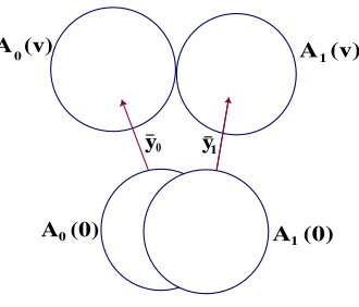
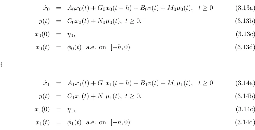
Thus, the output sets, Ai(v), are translates of open sets by ¯yi and they are affinely dependent upon the detection signal, v. We say a detection signal is proper if it gives disjoint output sets. That is, the detection signal v, is proper if the translation by the vector ¯yi pushes the sets apart. As we are looking for theminimum energy detection signal, then we will find a proper detection signal of minimum norm. Figure 1.3.1 illustrates a proper detection signal pushing the output sets apart. A detection signal is strictly proper if the output sets are a positive distance apart.
Formulating the problem in terms of the definition of proper
A (v)
y
A (v) 1
A (0) A (0)1
y
0 0
0 1
Figure 1.1: The figure illustrates a proper detection signal, v, pushing the output sets,
Ai(v), apart.
the noise bound. Recall that we assumed that the noise in the models was bounded. That is, we assumed
Si(xi(0), µi) =xi(0)TQixi(0) +
Z ω
0 |
µi(t)|2 dt <1, i= 0,1. (1.12)
Thus, if (x0, µ0, x1, µ1) satisfies the modelsandvis a proper detection signal,butan output,
y, is still in both output sets, it must be that
max{S0(x0(0), µ0),S1(x1(0), µ1)} ≥1. (1.13)
As this must be true for all possible (x0, µ0, x1, µ1) which satisfy the models but do not have distinct outputs, it is sufficient to ensure it is true for the minimum of them. Thus, we have
min xi,µi
max{S0(x0(0), µ0),S1(x1(0), µ1)} ≥1.
With this in mind, we can give a technical characterization of the term proper.
Lemma 1 (Proper Detection Signal). The auxiliary signal, v, is proper if and only if for all(x0, µ0, x1, µ1, y) satisfying
˙
x1 = A0x0+B0v+M0µ0
and
˙
x1 = A1x1+B1v+M1µ1
y = C1x1+N1µ1
then
min xi,µi
max{S0(x0(0), µ0),S1(x1(0), µ1)} ≥1. (1.16)
v is called not properif (1.16) does not hold.
The inner maximization is not continuous in the sense that it is over the discrete set i. Thus, the next step in formulating the optimal control problem which we will solve to find the test signal is to replace the discontinuous maximum problem with a continuous one and to switch the max and min (see Theorem 2.1 in [30]). That is, we replace
min xi,µi
max{S0(x0(0), µ0),S1(x1(0), µ1)} ≥1
with
max 0≤β≤1{minxi,µi
βS0(x0(0), µ0) + (1−β)S1(x1(0), µ1)} ≥1
Then finding the minimum energy, proper detection signal is equivalent to finding
minkvk2
such that
max 0≤β≤1xmini,µi
βS0(x0(0), µ0) + (1−β)S1(x1(0), µ1)≥1
subject to
˙
xi = Aixi+Biv+Miµi
y = Cixi+Niµi
fori= 0,1.
We note that the output y in both models is the same. Thus, we can eliminate the output by replacing
fori= 0,1 with
0 =C0x0−C1x1+N0µ0−N1µ1.
If we let
˙
x=Ax+Bv+M µ be
˙
x0 =A0x0+B0v+M0µ0 ˙
x1 =A1x1+B1v+M1µ1 and let
0 =Cx+N µ be 0 =C0x0−C1x1+N0µ0−N1µ1
then we can let
Jv(β) =
minxi,µiβS0(x0(0), µ0) + (1−β)S1(x1(0), µ1),
subject to
˙
x=Ax+Bv+M µ
0 =Cx+N µ.
Using these terms, the problem of finding the minimum energy detection signal becomes:
Find minkvk2
such that
max
0≤β≤1Jv(β)≥1.
The final step in the process of formulating the optimal control problem we will solve to find the minimum energy signal is to find the necessary conditions of theJv(β) problem. That is, we need to find
min xi,µi
βS0(x0(0), µ0) + (1−β)S1(x1(0), µ1) (1.18)
subject to
˙
x = Ax+Bv+M µ
0 = Cx+N µ.
Forming the Hamiltonian of this system, we get
H= 1 2x
T
0Qβx0+ 1 2µ
TV
where
1 2x
T
0Qβx0 =βx0(0)TQ0x0(0) + (1−β)x1(0)TQ1x1(0) (1.20) and
1 2µ
TV
βµ=βkµ0k2+ (1−β)kµ1k2. (1.21) Using the Euler equations, we get the necessary conditions
˙
x = Ax+Bv+M µ
˙
λ = −ATλ+CTη
0 = Vβµ−MTλ+NTη 0 = Cx+N µ
λ(0) = −Qβx(0), λ(ω) = 0.
Then the optimization problem for finding the minimum energy, proper detection signal is to minimize the detection signal subject to
1. An expression for the value of Jβ.
2. The necessary conditions for theJβ problem.
3. The constraintJβ ≥1.
This is equivalent to finding
minkvk2
subject to x˙ = Ax+Bv+M µ
˙
λ = −ATλ+CTη.
˙
Z = 1
2µ TV
βµ
0 = Vβµ−MTλ+NTη 0 = Cx+N µ
Z(0) = 1 2x
T
0Qβx0, Z(ω)≥1
The minimum energy detection signal algorithm (MEDS)
Having developed the optimization problem for solving the minimum energy detection sig-nal problem, we can now describe the algorithms and precise problems which are solved. Included with each step of the algorithm is the name of the software which can be used in that step. As we used MATLAB, by The MathWorks, Inc. [31], and SOCS, by The Boeing Company [7], they are given. However, other software packages would work just as well. In addition to MATLAB and SOCS, Maple, by Waterloo Maple, Inc. [49], was used to gener-ate the FORTRAN subroutines needed for SOCS. Note that the description below includes a change in variable resulting in a reduction of the dimensions of the problem and rewriting the Jv(β) problem in LQR form. As it added little to the understanding of the approach, these things weren’t mentioned above. However, they are included here for completeness. In [30], Horton includes a Riccati form of the problem but that is also not included here as we have not used it.
The minimum energy detection signal(MEDS) algorithm:
1. Perform QR decomposition onNiT (MATLAB)
NiT =QiRi
where theQi are unitary. Then
Ni=RTi QTi .
2. Perform constant orthogonal coordinate changes onµi (MATLAB).
(a) LetRTi =hNi 0
i
whereNi is invertible.
(b) LetQTi µi =
µi
e
µi
with the same partitioning asRTi . Thus,
Niµi =
h
Ni 0
i µi
e
µi
(c) LetMiQ−Ti =
h
MiMfi
i
with the same partitioning as RTi . Thus
Miµi =MiQ−ti QTi µi=
h
MiMfi
i µi
e
µi
.
Now, the system model is
˙
x = Ai+Bi+Miµi+Mfiµei (1.25a)
y = Cixi+Niµi. (1.25b)
3. Reduce model dimension by eliminatingy and µ0 (MATLAB).
(a) Combine both equations (i= 0,1) for y, solve for µ0, and substitute into (1.25) fori= 0. Then,
˙
x0= (A0−M0N −1
0 C0)x0+M0N −1
0 C1x1+B0v+Mf0eµ0+M0N −1 0 N1µ1.
(b) Let
x=
x0
x1
, A=
A0−M0N
−1
0 C0 M0N0−1C1
0 A1
, B =
B0
B1
,
M =
Mf0 M0N
−1
0 N1 0
0 M1 Mf1
, µ= µ0 µ1 e µi .
The system model is now
˙
x=Ax+Bv+M µ.
4. Compute new system matrices (MATLAB).
(a) Let C = hC0 −C1
i
and N =h0 N1 0
i
, with the columns of N conforming toµ.
(c) Let
R= 2
βI 0 0
0 (1−β)I+βNT1N1 0
0 0 (1−β)I
with the rows and columns ofR conforming to µ. (d) Compute A, B, M, H, Q, R.
5. Perform one of the following constrained optimization problems (SOCS)
(a) Problem formulation 1:
(γ∗)2 = max
v,β Z(ω) (1.30)
subject to the constraints
˙
x = Ax+Bv+M µ (1.31a)
˙
λ = −Qx−1
2Hµ−A
Tλ, λ0 =λω= 0 (1.31b) ˙
θ = vTv, θ(0) = 0, θ(ω) = 1 (1.31c) ˙
Z = 1
2[x
TQx+xTHµ+µTRµ], Z(0) = 0 (1.31d)
0 = Rµ+1 2H
Tx+MTλ (1.31e)
0.01< β <0.99. (1.31f)
(b) Problem formulation 2:
(γ∗)2= min v,β
Z ω
0 k
vk2dt
subject to the constraints
˙
x = Ax+Bv+M µ
˙
λ = −Qx−1
2Hµ−A
Tλ, λ(0) =λ(ω) = 0
˙
Z = 1
2[x
TQx+xTHµ+µTRµ], Z(0) = 0, Z(ω)
≥1
0 = Rµ+ 1 2H
Tx+MTλ 0.01< β <0.99.
1.3.2 Model Identification by the Separating Hyperplane
Applying the detection signal from the MEDS algorithm guarantees that the output sets from the models are distinct, convex sets. However, it does not reveal the model with which the output is associated. In order to determine from which model the output originated, other steps need to be taken. As we know that application of the detection signal causes the output sets to be disjoint and convex, we know that there exists a hyperplane separating them. Using this hyperplane, we can devise a test function, φ, and the identification can be made.
The Problem Let
˙
xi = Aixi+Bivˆ+Miµi (1.34a)
yi = Cixi+Niµi (1.34b)
fori= 0 and 1, be the previously defined normal and failed models with the exception that ˆ
v is now the minimum energy detection signal as found in the MEDS algorithm. Also, as we know that the minimum energy signal provides distinct output sets,y now has an index. Due to the design of the detection signal, we know that the output sets,Ai(v), are open, convex sets. We also know that while the output sets are distinct since we found a proper, minimum energy detection signal, the closures of the output sets are not distinct and must share at least one point. The reason for this is that the detection signal is minimal. If a detection signal which is infinitesimally smaller than the minimum energy detection signal were applied then the signal would not be proper and the output sets would not be disjoint. However, if the open output sets intersect with the application of an infinitesimally smaller detection signal, the closures of the output sets must intersect with the application of the minimum energy, proper detection signal.
a
y
y
y
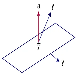
Figure 1.2: Using the hyperplane, a test can be formulated that will determine if y lies above the plane or below it, determining from which model the output is produced.
Let us assume there is a unique point of intersection. This is guaranteed if at least one of the sets is strictly convex. Also, recall that the equations y =Cixi+Niµi for i = 0,1 were combined to eliminate the y. Thus, when the optimal trajectory x1 and the optimal noiseµ1 are substituted into this expression, the resulting y is the point of intersection of the closures of Ai(v). Let the resultingy bey.
Because the output sets are convex and disjoint, there exists a hyperplane passing through y which separates the sets. Using this hyperplane, a test can be formulated such that it will determine if theylies above the plane or below it, thus determining from which model the output is produced. Figure 1.2 illustrates this. To state it more formally, there exists a function a(t) in L2 such that
φ(y) =ha, y−yi=
Z ω
0
a(t)T[y(t)−y(t)]dt (1.35)
and φ is non-negative on one output set and non-positive on the other. The function a(t) is the normal function to the separating hyperplane andφis called the test function.
As it is more numerically robust to work away from the boundary of the output sets, we improvise by artificially forcing the sets apart. Suppose that the points closest to each other on the sets arey0 and y1. Then the line segment between them would be defined by
We note here that a larger multiple of the minimum energy detection signal is still proper. More specifically, if v is proper, than (1 +c)v is also proper [30, 39], where c is some positive constant. Intuitively, if v pushes the output sets apart, then a detection signal larger than v will also push them apart. Any proper signal can be used to find the hyperplane.
We force the sets further apart by shrinking the noise components. This is equivalent to increasing the detection signal. To see this, consider the following system, where 0≤≤1:
˙
x = Ax+Bvˆ+M µ (1.36a)
y = Cx+N µ. (1.36b)
Multiplying this model by 1 and lettingz= x,w= y, andδ = 1, we get
˙
z = Az+Bδvˆ+M µ (1.37a)
w = Cz+N µ (1.37b)
which is the original model with the larger detection signal and no modification of the noise. Thus, we will use the model:
˙
xi = Aixi+Biˆv+Miµi (1.38a)
yi = Cixi+Niµi. (1.38b)
As we want the points on the boundaries of the closures of the sets which are closest to each other, we change the noise measure to
kµi k2≤1, i= 0,1. (1.39)
To compute the normal to the separating plane, we minimize k y0 −y1 k2 subject to (1.38) and (1.39). Then the difference of the solutions can be normalized and is normal to the hyperplane. We use the midpoint of the line segment between y0 and y1 as the point needed to define the hyperplane.
Model Identification Algorithm
2. Choose a value for <1.
3. Perform constrained optimization (SOCS)
minky0−y1k2 (1.40)
subject to the constraints
˙
xi = Aixi+Biˆv+Miµi (1.41a)
yi = Cixi+Niµi (1.41b)
˙
qi = µTi µi, qi(0) = 0, qi(ω)≤1 (1.41c)
fori= 0,1.
4. Lety0,and y1, be the closest points computed by the optimization.
5. Compute a(t) be the separating hyperplane (MATLAB)
a=
y0,−y1, ky0,−y1,k.
6. Compute y(t), the point on the separating hyperplane, as the midpoint, of the line segment connecting y0, and y1,(MATLAB)
y = y0,+y1,
2 .
7. Letφ(z) =ha, z−yi be the test function. Then
φ(y0) = ha, y0−yi>
φ(y1) = ha, y1−yi<
whereyi is an unknown output from model i,i= 0,1.
Numerical error increases due to division by small numbers, potentially effecting the results of the hyperplane test. This problem can be avoided the calculations are done to a sufficient level of accuracy. However, a suitable value ofwill also do. For a more detailed discussion of the choice of, see Chapter 3 in [30].
Multiple models
It is possible to find a detection signal with the MEDS algorithm which works for multiple models. Moreover, the model identification algorithm is applicable to multiple models, as well. When there are more than two models the output,y,may not come from either model being compared. Then the test becomes
ify∈
m
[
p=1
Ap(v), then
φi,j < i,j ⇒y6∈ Ai(v)
φi,j > i,j ⇒y6∈ Aj(v)
.
1.4
Outline of Thesis
In the chapter that follows, we explore the possibility of making the detection decision early. Then in Chapter 3, we introduce the delayed detection problem and look at solutions to it using the Method of Steps. With this background in the delayed detection problem, in Chapter 4, we look at a solution to the delayed detection problem by reformulating the problem into a partial differential equation (PDE) and then approximating the solution to the PDE with central differences. We look at another approximation in Chapter 5. This approximation adapts a spline method found in a paper by Ito and Kappel [34]. Then in Chapter 6, we look at some numerical examples. In the final chapter, we review some potentially interesting extensions to this work and give our conclusions.
1.5
Contributions of Thesis
The work done as part of this thesis appears in the following papers :
• S. Campbell, K. Drake, R. Nikoukhah, and F. Delebecque,Rapid Multi-Model Identi-fication In Systems With Delays, 3rd IFAC Workshop on Time Delay Systems (TDS
• S. Campbell, K. Drake, R. Nikoukhah, Early Decision Making When Using Proper Auxillary Signals, Proc. IEEE Conference on Decision and Control, Dec.10-13, Las Vegas, Nevada, 2002, pp. 1832-1837.
• S. Campbell, K. Drake, R. Nikoukhah,Auxillary System Design for Multimodel Iden-tification in Systems with Multiple Delays, Proc. 10th Mediterranean Conference on
Control and Automation, Lisbon, July 7-11, 2002.
• S. Campbell, K. Drake, R. Nikoukhah, Analysis of Spline Based Auxiliary Signal Design for Failure Detection in Delay Systems, Paper accepted by IEEE CSMC 2003.
• Kimberly J. Drake, An Examination of the Potential of Using the World Wide Web to Create User Interfaces , M&CT-TECH-00-013, December 2000, Mathematics and Computing Technology, A Division of the Boeing Co.
Early Detection
2.1
What is Early Detection and Why Bother?
We have,
˙
xi = Aixi+Bivˆ+Miµi (2.1a)
yi = Cixi+Niµi (2.1b)
for i = 0. . . m, for t ≥ 0 where xi, y, v, µi are the system states, output, detection signal and noise, respectively. Ai, Bi, Ci, Mi, Ni are matrices of appropriate dimension. v and µi are taken to be in L2[0, ω] = L2. This implies that xi and yi are in L2, as well. We also assume thatv is proper in the sense defined in Section 1.3 and that the output sets of the two models using this signal are distinct. According to the model identification algorithm of Section 1.3.2, we can then construct the hyperplane test function
φi,j(y) =< y−y¯i,j, a >=
Z ω
0
ai,j(t)T(y(t)−y¯i,j(t))dt
whereais a normal to a hyperplane between the output sets, ¯yis a point on the hyperplane, and [0, ω] is the test interval. As a and ¯y are computed offline, the hyperplane test is the calculation of a single integral which can be computed as the output,y, becomes available. Thus, the hyperplane test can be carried out in real time.
The question we wish to address in this chapter is whether it is necessary to wait until the end of the test interval to make the model identification decision. By developing a modified hyperplane test, based on the original test, we will show that it is possible to make
an early decision and computational tests will show that it is possible to reduce the time for the hyperplane test by about 25% on average and still maintain perfect model identification.
2.2
Analytical Breakdown of Problem
Assume we have the test function as described in Section 1.3.2
φi,j(y) =< y−y¯i,j, a >=
Z ω
0
ai,j(t)T(y(t)−y¯i,j(t))dt
where the test interval is [0, ω],ai,j(t)∈L2[0, ω] is the normal to the separating hyperplane and ¯yi,j is a point on the plane. We also assume that if φi,j(y) > i,j > 0 we know the output did not originate from model j. If φi,j(y) < i,j < 0, we know the output is not from modeli.
In the worst case, we may have to wait until the end of the interval in order to conclu-sively determine from which model the output originates. However, it is possible that we might be able to make this determination sooner. Let c ∈ [0, ω]. Let φi,j(y) =
ψi,j(y, c) + ∆i,j(y, c) where
ψi,j(y, c) =
Z c
0
ai,j(t)T(y(t)−yi,j(t))dt
and
∆i,j(y, c) =
Z ω
c
ai,j(t)T(y(t)−yi,j(t))dt.
Notice that ψi,j is the value of the hyperplane test function calculated until time c, as the output y becomes available, and ∆i,j is that part which is left to be calculated over the remaining test period [c, ω].
We have assumed that if φi,j(y)< i,j, we know the output is not from modeli. But, if
φi,j(y) =ψi,j(y, c) + ∆i,j(y, c) < i,j ⇒y6∈ Ai(v),
then
ψi,j(y, c) < i,j −∆i,j(y, c) ⇒y6∈ Ai(v).
0 2 4 6 8 10 12 14 16 18 20 0. 2
0 0.2 0.4 0.6 0.8 1 1.2 1.4
1.6 Resulting from Output from Model 2
Time
ψ2 ψ2
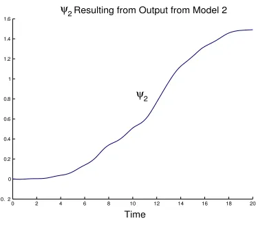
Figure 2.1: An example of ψi,j
In a worst case, we may not be able to make a decision until the end of the test interval. However, it is likely that we will be able to reach a decision earlier. Figure 2.1 shows ψi,j from an example we will discuss later in this chapter.
Let Lp(f) =R0T eAp(t−s)f(s)ds be the solution of ˙z=A
pz+f withz(0) = 0.Letxp(0) be the free initial condition for modelp. Using this notation, we have
y=CpLp(Bpv) + (CpLpMp+Np)µp+CpeApxp(0). (2.4) Then ∆ can be rewritten as
∆i,j(c) =
Z ω
c
aTi,j(CpLp(Bpv) +CpeApsxp(0)p+ (CpLM+Np)µp−y¯i,j) ds. (2.5) Notice that in estimating ∆i,j(y, c) a smaller estimate is available by grouping as many terms together as possible. That is,
∆i,j(c) =
Z ω
c
aTi,j(CpLp(Bpv) ds+
Z ω
c
aTi,j(CpeApsxp(0)) ds +
Z ω
c
aTi,j(CpLM +Np)µp −y¯i,j) ds.
Sm
p=1Ap(v). Let
δi,j(c) =
Z ω
c |
ai,j|2 ds
1 2
=kai,jkL2[c,ω] (2.7a)
Ki(c) = kCiLiMi+NikL2[c,ω] (2.7b)
γi,j,k(c) =
Z ω c
aTi,j(s) (CpLpBpv(s)−y¯i,j(s))ds
(2.7c)
θp(c) =
Z ω
c |
CpeApsQ−
1
2|2 ds
1 2
. (2.7d)
Then
1. If for some 0< t < ω we have that
ψi,j(y, t)> i,j + max
p [γi,j,p(t) + (Kp(t) +θp(t))δi,j(t)], then y6∈ Aj(v)
2. If for some 0< t < ω we have that
ψi,j(y, t)< i,j−max
p [γi,j,p(t) + (Kp(t) +θp(t))δi,j(t)], then y 6∈ Ai(v).
Proof. We know that
ify∈
m
[
k=1
Ap(v), then
φi,j < i,j ⇒y6∈ Ai(v)
φi,j > i,j ⇒y6∈ Aj(v).
together as possible. That is,
∆i,j(y, c) =
Z ω
c
aTi,j(CpLp(Bpv)−y¯i,j) ds+
Z ω
c
aTi,j(CpeApsxp(0)p) ds +
Z ω
c
aTi,j(CpLM+Np)µp ds
≤ k
Z ω
c
aTi,j(CpLp(Bpv)−y¯i,j) dsk+k
Z ω
c
aTi,j(CpeApsxp(0)p) dsk +k
Z ω
c
aTi,j(CpLpM+Np)µp dsk
≤ γi,j,p+k
Z ω
c
aTi,j(CpeApsxp(0)p) dsk+k
Z ω
c
aTi,j(CpLM+Np)µp dsk
≤ γi,j,p+
Z ω
c |
aTi,j|2 ds
1
2 "Z ω
c |
(CpeApsxp(0))|2 ds
1 2
+
Z ω
c |
(CpLM+Np)µp|2 ds
1 2
#
by the Cauchy-Schwartz inequality forL2
≤ γi,j,p+δi,j(θp+Kp) since kµk ≤1 and|Q−
1
2xp(0)|<1 by the noise measure
≤ max
p [γi,j,p+δi,j(θp+Kp)] since we don’t know what p is Then we have
φi,j(y) =ψi,j(y, c) + ∆i,j(y, c) < i,j ⇒y6∈ Ai(v)
so that
ψi,j(y, c) < i,j −∆i,j(y, c) ⇒y6∈ Ai(v).
But, since ∆i,j(y, c)<maxp[γi,j,p+δi,j(c) (θp(c) +Kp)], then
i,j−max
p [γi,j,p+δi,j(c) (θp(c) +Kp)] < i,j−∆i,j(y, c). Thus, if
ψi,j(y, c)< i,j−∆i,j(y, c) ⇒y6∈ Ai(v), then
ψi,j(y, c) < i,j−max
p [γi,j,p+δi,j(c) (θp(c) +Kp)] ⇒y6∈ Ai(v). Similarly, we have
so
ψi,j(y, c) > i,j−∆i,j(y, c) ⇒y6∈ Aj(v).
But, since
i,j−∆i,j(y, c) ≤ i,j+|∆i,j(y, c)|
≤ i,j+ max
p [γi,j,p+δi,j(c) (θp(c) +Kp)] then
ψi,j(y, c)> i,j+ maxp [γi,j,p+δi,j(c) (θp(c) +Kp)] ⇒y6∈ Aj(v).
♦
2.3
Algorithm
The theorem of the previous section shows that early decision making is possible. In this section, we provide the algorithm for the early decision test. We use standard numeri-cal packages in the numeri-calculations. As the quantities involve functions, we use differential equations in the calculations.
Calculating δi,j(c) =kai,jkL2[c,ω]
Let’s consider the function g(c) =kf(t)k2
L2[c,ω]=
Rω
c |f(t)|22 dt forc∈[0, ω]. First, we note thatg is monotonically decreasing on the interval [0, ω] and we note that g(0) =kfk2L2[c,ω]
whileg(ω) = 0.Then given values of the functionf, it is possible to computeg(c) by solving
˙
g=−|f(c)|22, g(0) =kfk22, 0≤t≤ω (2.14)
or
˙
g=−|f(c)|22, g(ω) = 0, 0≤t≤ω. (2.15)
As we haveai,j precalculated from the model identification algorithm, we can use (2.15) to calculate the valueδi,j(c) =kai,jkL2[c,ω]. That is, we solve
˙
g0 = −aTi,jai,j g(ω) = 0
δi,j = g
1 2
Calculating γi,j,k(c) =
RcωaiT,j(s) (CpLpBpv(s)−¯yi,j(s))ds
Using a similar technique as above, we can solve the following boundary value problem to find γi,j,k(c). As
γi,j,k(c) =
Z ω c
aTi,j(s) (CpLpBpv(s)−y¯i,j(s))ds
, we solve ˙
g1p(t) = Apg1p(t) +Bpv(t), g1p(0) = 0 ˙
g2p(t) = aTi,j(s) (Cpg1(t)−y¯i,j(s)), g2p(ω) = 0
γi,j,i(t) = |g2p|.
Calculating θp(c) =
R
ω
c |CpeApsP
−1 2 p |2 ds
1 2
The following initial value problem determines θp(c):
˙
g3p(t) = |CpeAptP −1
2
p |2, g3p(ω) = 0
θ(t) = g
1 2
3p(t).
Calculating Kp(c) =kCpLpMp+NpkL2[c,ω]
The Kp term is a bit more complicated. First, we note that separating the Mp and Np terms will make little difference computationally. Thus, we estimate kCpLpMpkL2[c,ω] and
kNpkL2[c,ω] separately. First,
kNpµkL2[c,ω] =
Z ω
c |
Np|22|µ|22 dt
1 2
≤ |Np|2
Z ω
c |
µ|22 dt
1 2
≤ |Np|2kµkL2[0,ω]
≤ |Np|2 since kµkL2[0,ω]<1.
AsNp is constant,|Np|2 is very easy to calculate. We can estimate kNpµkL2[c,ω]by finding
We also need to calculate estimates for kCpLp(Mpµ)kL2[c,ω]. First we show that there
existsMfp such that,
kCpLp(Mpµ)kL2[c,ω]≤Mfp(t)kµkL2[c,ω].
We know that
kLp(Mpµ)(t)kL2[c,ω]=
Z ω
c |
CpLp(Mpµ)(t)|22 dt
1 2
.
Lets consider a particular t∈[0, ω].Now,
|CpLp(Mpµ)(t)|2 ≤
Z t 0
CpeAp(t−s)Mpµ(s) ds
2
for t∈[0, ω]
≤
Z t
0 |
CpeAp(t−s)Mp|2|µ(s)|2 ds
by Cauchy-Schwartz Inequality ≤
Z t
0 |
CpeAp(t−s)Mp|22 ds
1
2Z t
0 |
µ(s)|22 ds
1 2
.
Now, let us consider |CpeAp(t−s)Mp|2.Since s≤tare both in [0, ω], we know thatt−s∈ [0, ω],so|CpeAp(t−s)Mp|2 =|CpeAptMp|2. Also, there exists an Mp(t) such that
|CpeAptMp|2≤Mp(t) for all t∈[0, ω]. Thus,
|Lp(Mpµ)(t)|2 ≤
Z t
0
Mp(s)2 ds
1
2 Z t
0 |
µ(s)|22 ds
1 2
=
Z t
0
Mp(s)2 ds
1 2
kµkL2[0,t] for t∈[0, ω].
Then letting Mfp(t)
1 2
=R0tMp(s)2 ds
1 2
,Mfp(t) will satisfy the differential equation,
˙
f
Mp(t) = M2p
f
Mp(0) = 1
whereMp =|CpeAptMp|2.Thus, we have for a particular tthat
|CpLp(Mpµ)(t)|2 ≤
f
Mp(t)
1 2
kµkL2[0,ω] since t∈[0, ω].
kCpLp(Mpµ)(t)kL2[c,ω] =
Z ω
c |
CpLp(Mpµ)(t)|22 dt
1 2 ≤ Z ω c f
Mp(t)12kµk
L2[0,ω]
2 dt 1 2 = Z ω c f
Mp(t)kµk2L2[0,ω]dt
1 2
= kµkL2[0,ω]
Z ω
c
f
Mp(t) dt
1 2
.
Note that to calculate RcωMfp(t) dt
1 2
, we can solve
˙
ff
Mp(t) = −Mfp ˙
f
Mp(t) = M2p
f
Mp(0) = 1
ff
Mp(ω) = 0
whereMp =|CpeAptMp|2.In order to calculate this, we needMp(t). There are several ways one might do this. For moderately sized problems, MATLAB offers several functions useful for calculating this value. The MATLAB function expm.m uses a Pad´e approximation to calculateeApt. expm2.m calculates the value ofeApt using a Taylor series. Also, MATLAB
provides expm3.m which calculates eApt by first diagonalizing A
pt. Once the value of eApt has been found, norm.m and normest.m can be used to find the value of|CpeAptMp|2.
Once the above quantities have been found, we can calculate Kp using ˙
f
Mp(t) = M2p, Mfp(0) = 1 ˙
ff
Mp(t) = −Mfp, fMfp(ω) = 0
Kp(t) = |Np|+Mff
1 2
p.
To summarize and state the above in a concise algorithm, we have the following:
1. Estimate Mp for p=0...m.
2. Estimate Kp for p=0...m.
Calculate Kp = kCpLpMp +NpkL2[c,ω] by calculating Mfp(t) =
Rt
0Mp(s)2 ds fMfp =
Rω
c Mfp(t) dt.
˙
f
Mp = M
2
p, Mfp(0) = 0 ˙
ff
Mp = −Mfp, Mffp(ω) = 0
Kp(t) = |Np|+Mffp
1 2
.
3. Estimateγi,j,p for p=0...m.
Calculate γi,j,k(c) =RcωaTi,j(s) (CpLpBpv(s)−y¯i,j(s))ds
using
˙
g1p(t) = Apg1p(t) +Bpv(t), g1p(0) = 0 ˙
g2p(t) = aTi,j(s) (Cpg1p(t)−y¯i,j(s)), g2p(ω) = 0
γi,j,p(t) = |g2p|.
4. Estimateθp(c) for p=0...m.
Calculate θp(c) =
R
ω c |Cpe
ApsP−
1 2
p |2 ds
1 2
with
˙
g3p(t) = |CpeAptP −1
2
p |2, g3p(ω) = 0
θ(t) = g
1 2
3p(t).
5. Estimate δi,j(c).
Useai,j to calculateδi,j(c) =kai,jkL2[c,ω]
˙
g0 = −aTi,jai,j g(ω) = 0
δi,j = g
1 2
0.
6. Estimateδbi,j(y,t).
Calculate
b
δi,j = max
(a) If for some 0< t < ω, we have that
ψi,j< i,j+bδi,j, then y6∈ Aj(v).
(b) If for some 0< t < ω, we have that
ψi,j(y, t)> i,j−bδi,j, then y6∈ Ai(v).
Note that if there are only two models, then the test becomes
1. If for some 0< t < ω, we have that
ψi,j < i,j+bδi,j, then y∈ Ai(v).
2. If for some 0< t < ω, we have that
ψi,j(y, t)> i,j−δbi,j, then y∈ Aj(v).
2.4
Computational Tests
In order to evaluate the early decision test, we ran 200 simulations using random noises and initial conditions. We considered the following 2-model example.
˙
x0 = −2x0+v+ (1 0)µ0
y = x0+ (0 1)µ0 ˙
x1 = −x1+v+ (1 0)µ1
y = x1+ (0 1)µ1 0≤t≤20.
We useQ0 =Q1 =I as the weight on the initial condition. In order to find random initial conditions and noises, we first generated on [−1,1] a set of random coefficients for the first 20 Fourier Sine functions and a random initial condition. We then normalized them onL2
0 2 4 6 8 10 12 14 16 18 20 8
6 4 2 0 2 4 6
8 100 Outputs from Model 1
δ
−δ
Time
0 2 4 6 8 10 12 14 16 18 20 8
6 4 2 0 2 4 6
8 100 Outputs from Model 2
Time
δ
δ −
Figure 2.2: When ψi,j, the value of the hyperplane test which is calculated as the output
y becomes available, crosses bδi,j or−bδi,j, the test is complete. In 100 trials on each model, detection takes place around .75ω.
0 10 20 30 40 50 60 70 80 90 100 14.4
14.6 14.8 15 15.2 15.4 15.6 15.8
16 Detection Times for Outputs from Model 1
Time
Trials 0 10 20 30 40 50 60 70 80 90 100
14 14.5 15
15.5 Detection Times for Outputs from Model 2
Time
Trials
True Solutions: The Method of Steps
3.1
Introduction to the Problem
Frequently, we assume that the future of a system is independent of past states and relies only on the present. This is not always a realistic representation of the systems under study. Models which are dependent on the past history of the state are common in many applications. For example, a model of measles spread in a city is given by
˙
S =−β(t)S[2γ+s(t−14)−S(t−12)] +γ (3.1)
withS(t) representing the susceptibles in the population at time tdays,γ representing the rate at which individuals enter the population, and β(t) representing a function charac-teristic of the population. An individual exposed at time t is infectious during the period [t−14, t−12] [27].
The circumnutation1 of sunflowers has been modelled by [27]
˙
α=−k
Z ∞
1
f(θ) sin(α(t−θ−t0))dθ (3.2)
whereα represents the angle the top of the plant makes with the vertical. The equation
˙
x=−αx(t−1)[1 +x(t)]
has been used to model the distribution of primes [27]. Later in this chapter, we will present an example of a model used in simulation of Mach number in a wind tunnel [48]. In each of
1
circumnutation: The successive bowing or bending in different directions of the growing tip of the stems of many plants, especially seen in climbing plants.
these cases, the past history of the system plays a vital role in its future. This past history enters the models in the form of delays, sometimes simply as a single, constant delay, as in the measles model (3.1), or sometimes in a more complex way, as in the model of the sunflower (3.2).
In this chapter, we consider detection on models with delays. The simplest of these models have the form:
˙
x = Ax(t) +Gx(t−h) +Bv(t) +M µ(t), t≥0 (3.3a)
x(0) = η, (3.3b)
x(t) = φ(t) a.e. on [−h,0) (3.3c)
y(t) = Cx(t) +N µ(t), t≥0. (3.3d)
This model illustrates some key similarities and differences between delayed models and models without delays. As usual, we take A, B, M, N, and C to be constant matrices to simplify discussion. G, the coefficient matrix of the delayed term, is also taken to be a constant matrix. Again,µis the noise andvis the detection signal. They are assumed to be functions inL2[0, ω],whereω is the detection horizon. Notice that rather than having just an initial condition, we have the addition of an initial function, φ∈ L2[−h,0), describing the past history of the state. In a delayed system, state space is infinite dimensional. This constitutes a significant difference from previously studied models and will require special handling in signal design.
Also, notice that we have no assumption of continuity between the initial function and the initial condition. That is, we do not assume that φ(0) = x(0). This will have ramifications when we consider the necessary conditions which we use as constraints in finding the detection signal.
There are two ways we can approach the fault detection question on such a model. One way would be to return to first principles, developing a new theory and a new signal design for this class of problems. While this is certainly possible, it is difficult in that we would need to consider optimal control on delayed systems. We need to determine the necessary conditions for (1.18) analytically in order to solve for the detection signal. This is a non-trivial task with a delayed system.
to one we have done before. By approximating these infinite dimensional systems by finite dimensional ones, we are able to extend previously developed theory to this new class of problems. There are technical and theoretical issues which must be addressed. However, the transition is smooth.
Among the technical and theoretical issues associated with this new class of problem is how the addition of this initial function, φ, is handled. Recall the noise measure in Section 1.3
Si(xi(0), µi) =xi(0)TQixi(0) +
Z ω
0 |
µi(t)|2 dt.
The initial condition,x(0), is included in the noise measure and treated as a disturbance of the system. Perfect detection is possible only because we bound the noise. Like the initial condition, the initial function will be treated as a disturbance and will contribute to the bounded noise. The noise measure becomes
Si(xi(0), φi, µi) =xi(0)TQixi(0) +
Z 0
−h|
φi(t)|2 dt+
Z ω
0 |
µi(t)|2 dt. (3.4)
Note that if ω < hthen (3.4) is actually
Si(xi(0), φi, µi) =xi(0)TQixi(0) +
Z ω−h
−h |
φi(t)|2 dt+
Z ω
0 |
µi(t)|2 dt. (3.5)
Also, ifω < h, then
˙
x = Ax(t) +Gx(t−h) +Bv(t) +M µ(t), t≥0 (3.6a) = Ax(t) +Gφ(t−h) +Bv(t) +M µ(t), for allt∈[0, ω]. (3.6b)
Since φis considered a disturbance, then (3.6b) can be rewritten as
˙
x = Ax(t) +Bv(t) + ˜Mµ˜(t), t≥0
where ˜M = [G M] and ˜µ =
φ
µ
. The problem has been rewritten without delays and
requires no further special care. Thus, we will only consider the case whenω > h.
4. Finally, we look at a direct approximation using splines, as is discussed in Chapter 5. Approximations allow for more complicated models than the Method of Steps. However, the Method of Steps provides a true solution, rather than an approximate one. Thus, solutions using the Method of Steps serve as a basis of comparison and verification of the other two methods.
3.2
True Solutions with the Method of Steps
In this section, we will introduce the Method of Steps. By breaking up the detection horizon into pieces which are the length of the delay and assigning to those pieces a new variable, the delay term can be eliminated from the system. With a few modifications, the theory of previous chapters will apply. Unfortunately, while the Method of Steps provides a true solution, it only works on a small class of problems.
3.2.1 The Basic Problem
A simple illustrative example
In order to motivate the ideas behind the Method of Steps, we first consider a simple example. Suppose we wish to find a continuous solution to the differential delay equation (DDE) given by
˙
x(t) = x(t−1) (3.8a)
x(t) = φ= 1 for −1< t≤0. (3.8b)
Then if (3.8) is to hold for 0< t≤1, we need
˙
x(t) = x(t�