Building Structures under Pressurization of High Energy Line Break – Linear Analysis

(1)

Building Structures under Pressurization of High-Energy Line Break –

Linear Analysis Method

Taha D. AL-Shawaf1

1

Manager, Material and Structural Analysis, AREVA NP Inc, Naperville, IL

ABSTRACT

In this paper a simplified linear method for evaluating building structures under pressurization of high-energy line break (HELB) is presented. The method numerically calculates the dynamic load factors using spread-sheet software. Typically, a dynamic load factor (DLF) value of 2.0 was traditionally used for evaluating a structure under an impulse load. This paper shows that some irregular pressure-time histories may produce a DLF that is greater than 2.0. Calculating the fundamental frequency of a structural component often lowers the DLF thus reducing the applied maximum equivalent pressure.

INTRODUCTION

Design Basis Specifications for most nuclear power plants require that rooms or compartments that are affected by the post-accident pressure of HELB be designed and constructed to minimize or resist this pressure. Some rooms contain blowout panels that restrict the potential internal compartment over-pressure due to pipe rupture. An evaluation of the various structural components in any given room is required for the pressure transient that is exerted in that room. Recently, some utilities have re-evaluated this loading due to revised predicted failure pressure of the blowout panels, increased pressure due to power uprate, or new steam generator installation.

Class 1 Structures are required to resist effects of jet impingement (if any), flooding, and sub-compartment pressurization. Jet impingement is not part of the scope of this paper. Flooding takes more time for the water to reach its maximum height; i.e., is a slowly applied load. Hence, flooding can be considered as a static load and can be evaluated simply. This paper uses linear analysis techniques to determine the capacities of the various structural components and evaluate them against the internal pressurization loading resulting from a HELB.

Compartment pressurization is considered an impulse load since it is a transient(time varying)load determined by an external source and is relatively insensitive to the structural response. The pressure-time history is calculated using thermal-hydraulics system simulation software and is not part of the scope of this paper. A given room may have several volumes. Each volume may be subjected to a pressure-time history that is different than an adjacent volume.

METHODOLOGY

In general the pressure-time history curve is irregular. Several methods can be used in this dynamic analysis. A finite element dynamic analysis may be used to compute the response of the generally non-linear pressure-time history at any volume. Modeling every structural component and performing a dynamic finite element analysis can be very time consuming and expensive.

Calculating a dynamic load factor (DLF) for each of the time history curves is much simpler. The DLF concept is a well known method[1] in which a factor (DLF) is calculated and represents the ratio of the peak dynamic response, PDyn, of a

single degree of freedom (SDOF) structure to the static response, Pstat, to the maximum pressure-time history.

PDyn = (DLF) Pstat (1)

The DLF, also known as dynamic magnification factor, depends on the frequency of the SDOF. Since deflections, internal forces, and stresses in an elastic system are all proportional, one can write

DLF = xm / xs (2)

where:

xs = static deflection or, in other words, the displacement produced in the system when the peak load is applied statically

xm = maximum dynamic deflection

(2)

Reference [1] shows DLF versus td/T for a number of simple force time history inputs, see Fig 1. The impulse length ratio, also known as duration ratio, is the ratio of the impulse duration to the natural period of the structure, or td/T. It is important to note that, for an impulse of short duration, a large part of the applied load is resisted by the inertia of the structure and the stresses produced are much smaller than those due to the longer duration loading. For the most prevalent load cases, namely, the isosceles triangular load and the rectangular load forcing function, the maximum values of DLF are 1.52 and 2.0, respectively [1]. This immediately indicates that all maximum displacements, forces, and stresses due to the dynamic load are twice the value that would be obtained from a static analysis for the maximum load, Pstat.

0 0.5 1 1.5 2 2.5

0 0.5 1 1.5 2 2.5 3 3.5 4

td/T

DL

F Rectangular

Triangular

Rectangular Forcing Function

td F1

Isosceles Triangle Forcing Function td F1

Fig. 1 Maximum Response of SDOF (undamped) Subjected to Rectangular and Triangular Forcing Functions

Hence, the dynamic analysis is transformed into a static analysis by applying the maximum load multiplied by the DLF associated with the fundamental frequency of the structure. Here, there is an assumption that the structure is behaving essentially as a SDOF structure. For our case, in which a pressure is applied on walls and slabs, the predominant behavior is the fundamental mode response. It is common to use a DLF of 2 to represent the maximum response for a predominantly triangular pulse loading. However, as will be seen later, DLF’s higher than 2 are possible. In the design of structures subjected to impulse loads, the first peak of response is usually the only cycle of response that is of interest since the maximum resistance and deflection is attained in that cycle. In general, damping has little effect on this first peak. However, structural damping has some effect on the subsequent response of the structure.

One way to find the DLF for an arbitrary force-time history curve is by analyzing a number of SDOF systems each having a different frequency and plotting the maximum response against the frequency for each SDOF system. This may be an iterative process since it is not known at what frequency the maximum response will occur or more SDOF systems may be analyzed at closer frequencies in order to capture the maximum response. This paper uses a numerical method to compute the response of an irregular forcing function.

Reference [2] provides one of the methods that uses piecewise-linear interpolation of the forcing function within a time step Δt. The resulting equations for the response (displacement and velocity) at the end of time step j are:

(3)

⎥ ⎦ ⎤ ⎢ ⎣ ⎡ Δ ⎟⎟ ⎠ ⎞ ⎜⎜ ⎝ ⎛ + Δ + ⎥ ⎥ ⎦ ⎤ ⎢ ⎢ ⎣ ⎡ ⎭ ⎬ ⎫ ⎩ ⎨ ⎧ Δ + ⎥ ⎥ ⎦ ⎤ ⎢ ⎢ ⎣ ⎡ ⎭ ⎬ ⎫ ⎩ ⎨ ⎧ Δ + Δ Δ Δ = • • Δ − Δ − Δ − • ) t sin( x x -) t cos( x ) t sin( F ) t sin( ) t cos( -1 t k F x j 1 -j 1 -j j 1 -j t j 2 t 1 -j j j t j j j j j j d n d n d d d n d d n d n n n e e k e ω ξ ω ω ξω ω ω ω ω ω ω ξω ω ξω ξω ξω (4) where:

Fj = Force at time step j k = stiffness

Δ = Designates change in a quantity during the time step

ωn = Natural frequency of the SDOF system in radians/sec

•

x = velocity x = displacement

ωd = Natural frequency of damped SDOF system in radians/sec

= ωn SQRT (1-ξ2) ξ = damping ratio

For our purposes, the initial conditions at time = 0.0

0.0 x and 0.0

x = =

•

(5)

If the maximum displacement, x, from all time steps is xm and the static displacement is xs (which is equal to the peak force divided by k), then the DLF = xm/xs.

In order to calculate the DLF for a specific reinforced concrete component (e.g., slab), it is necessary to find the stiffness of the component. Since the stiffness calculation is complicated by the fact that the moment of inertia of the cross section changes continually as cracking progresses, it has been recommended (References [4] and [5]) that the average moment of inertia, Ia, be used, [4] and [5].

Ia = (Ig+Ic)/2 (6)

where: Ig = 1/12 b tc

3

= the gross moment of inertia Ic = Fbd3 = the cracked moment of inertia b = the width of the element (for slabs, b is

taken as unit width)

tc = total (gross) thickness

d = distance from the extreme compression fiber to centroid of tension reinforcement.

F = Coefficient given in Fig. (2) (from [4] and [5])

0 0.01 0.02 0.03 0.04 0.05 0.06 0.07

0 0.004 0.008 0.012 0.016 0.02

Reinforcement Ratio As/bd

Co

efficent F

n = 10 n = 8 n = 6

(4)

For one-way members, the reinforcement ratio, ρ, used to obtain the factor F should be an average of the tension steel at the supports and midspan. Similarly, the effective depth, d, used to compute the cracked moment of inertia is the average of the effective depth at the mid span and the supports.

For two-way members, the above is repeated in the length and width directions to obtain the cracked moment of inertia ICL and ICW, respectively. The combined effective cracked moment of inertia for the slab is then calculated by considering the aspect ratio of the slab, [4]:

W L

W I L I I_c CL CW

+ +

= (7)

where:

ICL = cracked moment of inertia in the plane along the length direction

L = span length

ICW = cracked moment of inertia in the plane along the width direction

W = span width

The equivalent thickness can then be calculated

3 a

e

b I 12

t = (8)

Use te and the distributed dead load mass (including equipment weight) to find the natural frequency of the component.

MATERIAL BEHAVIOR

Material properties (e.g., yield strength) are subject to statistical and dynamic variation. Statistical variations are defined as the difference between the minimum code specified value and the higher actual value, which ranges between 10-25 percent for the yield strength of steel and 10 to 30 percent for the compressive strength of concrete, [5].

The dynamic variation is due to the increase in strain rate and increases the yield stress of steel and compressive strength of concrete. These increases must be accounted for to conservatively predict reaction or pass-through loads from a structural element affected by impulse load. It is common to take credit for the dynamic strength increase, but not the statistical increase, in designing the affected element itself.

Reference [5] provides recommended values of dynamic increase factors (DIF) for use in design. Reference [6] gives the limits on DIF’s for concrete and reinforcing steel. Material properties considered in determining resistance to impulse loads are found by multiplying the static values by the appropriate DIF.

IMPLEMENTATION

The method described in the previous section lends itself to be programmed using spreadsheet software. Table 1 shows the application of this method for an isosceles triangular forcing function. Figure 3 shows a plot of the loading function and the displacement response time history as well as the DLF plot for the same triangular forcing function. Note that the maximum displacement occurs after the maximum peak loading. The DLF curve agrees with that reported in Reference [1] and also shown in Figure 1. These results are for essentially undamped (Damping = 0.01percent) SDOF system.

Force and Response Time History

-2.5 -2 -1.5 -1 -0.5 0 0.5 1 1.5 2 2.5

0.0 0.5 1.0 1.5 2.0 2.5 3.0

Time

For

c

e

or

D

is

p

la

c

e

ment

Force Displacement

a. Force-Time History and Resulting Displacement

Maximum Response of SDOF System Triangular Forcing Function

0 0.2 0.4 0.6 0.8 1 1.2 1.4 1.6

0 0.5 1 1.5 2 2.5 3 3.5

Td/T

DLF

b. DLF vs. td/T Fig. 3 Triangular Forcing Function

(5)

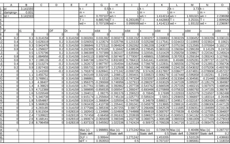
Table 1. Solving for DLF for a Triangular Forcing Function

1 2 3 4 5 6 7 8 9 10 11 12 13 14 15 16 17 18 19 20 21 22 23 24 25 26 27 28 29 30 31 32 33 34 35 36 37

A B C D E F G H I J K L M N O

pi 3.141593 k = 0.5 k = 1 k = 2 k = 3.73 k = 5

damping= 0.001 m = 1 m = 1 m = 1 m = 1 m = 1

td = 3.141593 wn = 0.707107 wn = 1 wn = 1.414214 wn = 1.931321 wn = 2.236068 T = 8.885766 T = 6.283185 T = 4.442883 T = 3.25331 T = 2.809926 wd = 0.707106 wd = 0.999999 wd = 1.414213 wd = 1.93132 wd = 2.236067

F t1 t DF Dt x xdot x xdot x xdot x xdot x xdot

0 0 0 0 0 0 0 0 0 0 0 0 0 0 0

0.2 0.1 0.314159 0.2 0.314159 0.003281 0.031282 0.003273 0.031152 0.003257 0.030893 0.003229 0.030452 0.003209 0.030131 0.4 0.2 0.628319 0.2 0.314159 0.026055 0.123574 0.025796 0.121533 0.025288 0.117541 0.024433 0.110893 0.023824 0.10621 0.6 0.3 0.942478 0.2 0.314159 0.086846 0.272312 0.084924 0.262262 0.081209 0.243077 0.075156 0.212565 0.070994 0.192173 0.8 0.4 1.256637 0.2 0.314159 0.202305 0.470165 0.19442 0.439535 0.179545 0.383103 0.156394 0.299169 0.14129 0.24733 1 0.5 1.570796 0.2 0.314159 0.386389 0.707388 0.363107 0.635984 0.320581 0.510429 0.258258 0.339827 0.220342 0.245624 0.8 0.6 1.884956 -0.2 0.314159 0.643113 0.909745 0.587467 0.770067 0.489801 0.538569 0.357053 0.259184 0.283243 0.127681 0.6 0.7 2.199115 -0.2 0.314159 0.946738 1.004751 0.832483 0.766413 0.641441 0.400381 0.40486 0.025281 0.287737 -0.110761 0.4 0.8 2.513274 -0.2 0.314159 1.262672 0.987787 1.054594 0.625466 0.726678 0.122831 0.365556 -0.278248 0.212851 -0.356706 0.2 0.9 2.827433 -0.2 0.314159 1.555731 0.859737 1.212508 0.361104 0.709619 -0.240088 0.234139 -0.543032 0.075206 -0.493765 0 1 3.141593 -0.2 0.314159 1.791873 0.626941 1.271242 -0.000725 0.57426 -0.617867 0.038477 -0.674651 -0.078908 -0.457237 0 1.1 3.455752 0 0.314159 1.943149 0.332165 1.208812 -0.393401 0.330823 -0.906278 -0.167448 -0.595858 -0.192261 -0.23452 0 1.2 3.769911 0 0.314159 1.998881 0.0212 1.028132 -0.747334 0.023397 -1.018543 -0.313384 -0.304581 -0.21448 0.098856 0 1.3 4.08407 0 0.314159 1.956375 -0.290668 0.746956 -1.027913 -0.288297 -0.933029 -0.347339 0.095007 -0.135179 0.384987 0 1.4 4.39823 0 0.314159 1.817761 -0.588116 0.392862 -1.207728 -0.543762 -0.666509 -0.257335 0.460215 0.007975 0.488546 0 1.5 4.712389 0 0.314159 1.589895 -0.856535 0.000547 -1.269247 -0.693466 -0.270869 -0.075632 0.660792 0.147155 0.360787 0 1.6 5.026548 0 0.314159 1.284011 -1.08275 -0.391576 -1.206523 -0.70845 0.17699 0.132833 0.625379 0.216507 0.062488 0 1.7 5.340708 0 0.314159 0.915174 -1.255664 -0.745134 -1.025773 -0.585924 0.5901 0.293655 0.366897 0.183314 -0.26496 0 1.8 5.654867 0 0.314159 0.501534 -1.366804 -1.025554 -0.744758 -0.34979 0.888317 0.349517 -0.022167 0.063426 -0.466574 0 1.9 5.969026 0 0.314159 0.063435 -1.410738 -1.205441 -0.391041 -0.045979 1.013865 0.280616 -0.402851 -0.086306 -0.447128 0 2 6.283185 0 0.314159 -0.377586 -1.385336 -1.267255 0.00072 0.266486 0.942529 0.111685 -0.639351 -0.194989 -0.216136 0 2.2 6.911504 0 0.628319 -1.182643 -1.134986 -1.024908 0.744988 0.684919 0.300767 -0.270639 -0.42458 -0.127534 0.394007 0 2.4 7.539822 0 0.628319 -1.757458 -0.66458 -0.391632 1.203939 0.596927 -0.561914 -0.300501 0.341162 0.152395 0.345428 0 2.6 8.168141 0 0.628319 -1.990674 -0.065609 0.390346 1.202739 0.068375 -1.008198 0.060033 0.661909 0.177418 -0.279019 0 2.8 8.796459 0 0.628319 -1.837333 0.545562 1.022336 0.742424 -0.50972 -0.709328 0.341716 0.122119 -0.093475 -0.436448

1 Max (x) 1.998881 Max (x) 1.271242 Max (x) 0.726678 Max (x) 0.40486 Max (x) 0.287737 Static defl. 2 Static defl. 1 Static defl. 0.5 Static defl. 0.268097 Static defl. 0.2 DLF = 0.99944 1.271242 1.453355 1.510126 1.438683 td/T = 0.353553 0.5 0.707107 0.965661 1.118034

The same methodology and essentially the same spreadsheet were used to obtain the DLF for the pressure-time histories at different volumes/compartments that are subjected to HELB. For these cases, however, the appropriate damping ratios are used for reinforced concrete and steel structures. The pressures can also be considered as a force applied on a unit area. The typical pressure-time history curve has its highest magnitude of the pressure occurring within the first 1.0 sec. Hence, the time histories from time equal 0.0 to 1.0 second were used in the DLF spread sheets. The frequency (i.e., the stiffness and mass) are varied to obtain the associated DLF. It should be noted that the response at a time step is calculated at the end of that time step, i.e., the potential exists that the maximum response may occur at the middle of the time step and may be missed. This numerical error may occur if the time step is relatively large or at sudden changes of the input pressure-time history. However, the pressure-time step of the pressure-pressure-time history is sufficiently small; and by inspecting the resulting displacement-time history plots, no sudden variation or change is shown. Hence, this numerical error is not present. On the other hand, the peak response is sensitive to the frequency of the SDOF system. So the stiffness or the mass are manually selected in the spread-sheet to be near the peak frequency in order to ensure the maximum DLF is captured.

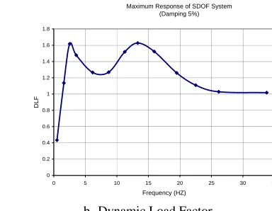
Typical pressure-time history transients and the DLF curves are shown on Figures 4 to 7. As expected the amplitude of the response for low natural frequency is higher than that for higher frequency. Note that in some cases the peak response may occur at the second cycle of vibration as shown in Figure 4. Figure 4 also shows a double peak for the DLF curve. The second peak occurs at around 13Hz, which is close to a typical fundamental frequency of a concrete slab. Figure 5 shows a maximum DLF greater than 2.0. This is due to the successive application of the two peaks in the forcing function that amplify the response.

The two peaks in the DLF curve that are present in Figure 4 are combined to form one large plateau that extends between approximately 3 to 14 Hz as shown in the example of Figure 6. Figure 7 on the other hand show distinct three peaks in the DLF curve. From these examples, it is recognized that the shape of the forcing function and the fundamental frequency of the structure plays a major role in defining the DLF and thus the maximum load that the structure is subjected to.

(6)

-1 -0.5 0 0.5 1 1.5 2 2.5 3 3.5 4

0.0 0.1 0.2 0.3 0.4 0.5 0.6 0.7 0.8 0.9 1.0

Time (sec)

F

o

rc

e or

Pr

es

s

u

re

-0.04 -0.02 0 0.02 0.04 0.06 0.08 0.1 0.12 0.14 0.16

Disp

la

c

e

m

e

n

t

Force 0.503 Hz 2.516 Hz

a. Force-Time History and Resulting Displacements for Different Fundamental Frequencies

Maximum Response of SDOF System (Damping 5%)

0 0.2 0.4 0.6 0.8 1 1.2 1.4 1.6 1.8

0 5 10 15 20 25 30 35

Frequency (HZ)

DL

F

b

.

Dynamic Load Factor

Fig. 4 Results showing DLF less than 2

-0.5 0 0.5 1 1.5 2 2.5

0.00 0.10 0.20 0.30 0.40 0.50 0.60 0.70 0.80 0.90 1.00

Time (sec)

For

c

e or

P

re

s

ur

e

-0.0025 -0.0015 -0.0005 0.0005 0.0015 0.0025 0.0035

Disp

la

ce

m

e

n

t

Force 7.12 Hz 5.96 Hz

Maximum Response of SDOF System (5% Damping)

0 0.5 1 1.5 2 2.5

0 5 10 15 20 25 30 35

Frequency (HZ)

DLF

b

.

Dynamic Load Factor

Fig. 5 Results showing DLF greater than 2

-0.5 0 0.5 1 1.5 2 2.5 3

0.00 0.10 0.20 0.30 0.40 0.50 0.60 0.70 0.80 0.90 1.00

Time

F

orc

e or

Pr

es

s

ur

e

-0.0002 0 0.0002 0.0004 0.0006 0.0008 0.001 0.0012

Disp

la

ce

m

e

n

t

Force 9.42 Hz 14.06 Hz

0 0.2 0.4 0.6 0.8 1 1.2 1.4 1.6 1.8

0 5 10 15 20 25 30 35

Frequency (HZ)

DLF

b

.

Dynamic Load Factor

(7)

-0.5 0 0.5 1 1.5 2 2.5

0.00 0.20 0.40 0.60 0.80 1.00

Time (sec)

F

o

rc

e or

P

re

s

u

re

-0.012 -0.008 -0.004 0 0.004 0.008 0.012

D

is

pl

ac

e

ment Force 7.47 Hz 2.76 Hz

0 0.5 1 1.5 2 2.5

0 5 10 15 20 25 30 35

Frequency (HZ)

DLF

b

.

Dynamic Load Factor

Fig. 7 Results showing Three Peaks in the DLF Curve

EVALUATION PROCESS

The DLF curves are generated for each pressure-time history associated with a specific volume. Given the natural frequency of a component subjected to a pressure associated with a particular volume, the DLF can be obtained from the curve for that volume. The DLF is multiplied by the maximum pressure of this volume to obtain the maximum equivalent static pressure to be used in evaluating the component. The evaluation determines whether the maximum allowable pressure (capacity) that the component can withstand bounds the pressure-time histories, including the DLF.

The first step in determining the HELB pressure capacity of a slab or wall is to determine the ultimate bending moment capacity of that concrete component (ΦMn). Note that the contribution of compression steel to the moment capacity is conservatively ignored. This moment capacity is multiplied by a DIF due to the rapid application of the HELB pressure load.

In most cases, the slabs and walls were designed as one-way members. Because of this, the pressure capacity of the components could be determined using traditional beam equations (e.g. simply supported beam, fixed-fixed beam, cantilever and propped cantilever beams) and solving for the uniform load.

The slab loading is a factored load that includes the self weight of the slab. The live load such as equipment load are considered part of the dead load. For the slabs (floors) at the bottom of the volume under consideration, the HELB pressure is pushing down on the slab; so the self weight load acts in the same direction and reduces the allowable HELB pressure load. However, for slabs (ceilings) at the top of the volume under consideration, the HELB pressure will push up on the slab. Thus, the weight of the slab will increase the pressure capacity of the slab. In this case the load factor associated with the dead and live load is taken as 1.0. For the case of the concrete walls, self weight will not have any effect. The load factors to be used for the HELB pressure load and the dead load (e.g., concrete slab weight) depends on the licensing commitment of the plant. However, it may be argued that since the pressure-time histories are determined by extensive thermal hydraulics simulation software, there is less uncertainty in the pressure values. Hence, accidental pressure load factor may be reduced provided license documents are updated with the approval of the regulators.

In general, evaluations of reinforced concrete slabs and walls show that shear capacity does not control. The bending capacity for a unit width of a reinforced concrete slab is calculated as follows:

DIF ' c 2(0.85)f

AsFy d

AsFy bend Φ

ΦMn _⎟⎟

⎠ ⎞ ⎜

⎜ ⎝ ⎛

−

= (9)

where:

Φ = capacity reduction factor Mn = nominal bending strength Φ Mn = design flexural strength Φbend = 0.9

As = area of tension reinforcement within the width Fy = Minimum yield stress of tension reinforcement fc’ = concrete compressive strength

(8)

Compute failure load for a simply supported beam in which the dead and live loads acting in the same direction of the pressure,

design 2

u ) w

L ΦMn (8

w = − (10)

And for dead and live load acting opposite to the pressure:

design 2

u w

L ΦMn 8

w ⎟+

⎠ ⎞ ⎜ ⎝ ⎛

= (11)

where:

L = span of the simply supported beam wu = ultimate load for the slab

wdesign = design load for the slab = LFDL (Dead Load + Live Load)

LFDL = load factor for dead load

The allowable unfactored pressure, Pall, can then be computed by dividing by the load factor of accidental pressure, LFp

p u all

LF w

P = (12)

The allowable pressure, Pall, is the capacity of the reinforced concrete slab. For a steel structure, using the allowable stress design method and DIF, the capacity (in units of pressure) of the structure under uniform pressure is calculated. The structure is qualified if its capacity exceeds that of DLF multiplied by the Peak Pressure.

SUMMARY AND CONCLUSIONS

A detailed linear method is presented to evaluate building structures under HELB pressurization loads. Maximum dynamic load factors of 2.0 or less are typical however in some cases higher than 2.0 may be found for certain force-time histories and at relatively low frequencies. Calculating the fundamental frequency of a structural component often lowers the DLF thus reducing the applied maximum equivalent pressure. For evaluation of ceiling slabs, the dead load and live load act opposite to the pressure and thus a load factor of 1.0 is used. Accidental pressure load factor may be reduced to account for the added certainty of the load definition if calculated using thermal-hydraulics simulation software.

REFERENCES

1. Biggs, J. M., Introduction to Structural Dynamics, McGraw-Hill Book Co., 1964. 2. Rao, S. S., Mechanical Vibrations, Addison-Wesley, 2nd Edition, 1990.

3. Dede, M., Sock, F., Lipvin-Schramm, S. and Dobbs, N., “Structures to Resist the Effects of Accidental Explosions”- Volume III, Principles of Dynamic Analysis, AD-148895, Ammann & Whitney, New York June 1984.

4. Dede, M. and Dobbs, N., “Structures to Resist the Effects of Accidental Explosions”, Volume IV, Reinforced Concrete Design, AD-A178901, Ammann & Whitney, New York April 1987.

5. ASCE “Structural Analysis and Design of Nuclear Plant Facilities”, Manuals and Reports on Engineering Practice – No. 58, American Society of Civil Engineers, New York 1980.