The Initiation and Evolution of Multiple Modes of Convection Within a Meso-Alpha Scale Region

(1)

ABSTRACT

FRENCH, ADAM JAMES. The Initiation and Evolution of Multiple Modes of

Convection Within a MesoAlpha Scale Region. (Under the direction of Matthew D. Parker.)

(2)

(3)

The Initiation and Evolution of Multiple Modes of Convection

Within a MesoAlpha Scale Region

by

ADAM JAMES FRENCH

A thesis submitted to the Graduate Faculty of North Carolina State University

in partial fulllment of the requirements for the Degree of

Master of Science

Marine, Earth, and Atmospheric Sciences

Raleigh, North Carolina 2007

APPROVED BY:

Matthew D. Parker, Chair of Advisory Committee

(4)

Dedication

To the men and women of my generation, and of generations past who instead of spending their late teens and early twenties pursuing higher education and enjoying college life, spent them around the world protecting our freedom. Without you, none of

(5)

Biography

Adam French was born and raised in Manchester, Connecticut where he got to expe-rience a wide variety of weather, from summer thunderstorms to winter nor'easters. This sparked an interest in the weather at an early age, however it was not until he wrote his 11th grade honors thesis on severe weather in Connecticut that Adam decided he wanted to become a meteorologist.

Adam attended Valparaiso University in northern Indiana from 2001-2005, where he received his B.S. in meteorology. While at Valpo, Adam was also a member of Christ College, an interdisciplinary honors college, from which he earned a minor in humanities, and graduated as a Christ College scholar. In the summer of 2004, Adam participated in the National Weather Center Research Experience for Undergraduates in Norman, Oklahoma where he analyzed data from the SPC/NSSL Spring Program. During his senior year at Valpo, Adam served as president of the Northwest Indiana Chapter of the National Weather Association and played a main role in the organization and running of the 3rd Annual Great Lakes Meteorology Conference. Following graduation from Valparaiso in 2005, Adam came to North Carolina State University and began pursuing a Masters degree as one of the inaugural members of the Convective Storms Group under Dr. Matthew Parker.

(6)

Acknowledgments

(7)

List of Figures

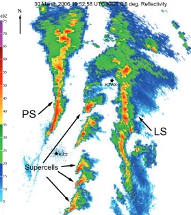
1.1 Extended range base reectivity from Wichita, Kansas at 1957 UTC 30 March 2006. Three modes of convection (PS, supercell, LS) are labeled for reference. . . 4 1.2 Storm reports received by the Storm Prediction Center in Norman,

Okla-homa between 1800 UTC 30 March 2006 and 0000 UTC 31 March 2006. Green dots denote hail reports, blue pluses severe wind, and small red crosses or lines denote tornadoes and tornado tracks. Numbers plotted next to tornado reports refer to Fujita scale intensity rating. Blue outline signies storm reports associated with the PS squall line, with the dashed blue indicating reports during and after transition to the TS structure. Red outline signies reports associated with supercells. . . 5

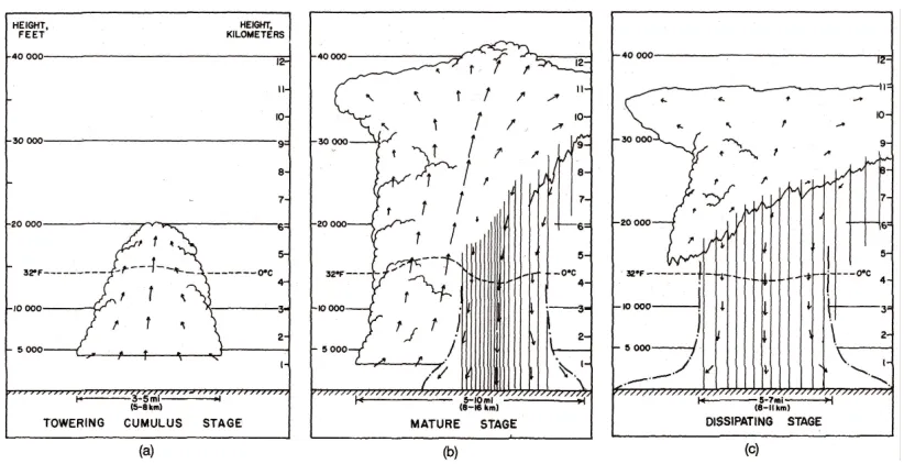
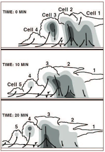
2.1 Life cycle of an ordinary cell thunderstorm: a)towering cumulus stage dominated by updrafts, b) mature stage containing updrafts and down-drafts, c) dissipating stage dominated by downdrafts (adapted from Byers and Braham, 1949). . . 22 2.2 Cross section through a multicell storm over the course of 20 minutes.

(10)

2.3 Schematic of a supercell thunderstorm noting the location of prominent updrafts, downdrafts and airows as well as outlining a typical radar sig-nature (from Lemon and Doswell, 1979). . . 24 2.4 The eects of wind shear and cold pool induced circulations on a squall

line updraft. a) No shear or cold pool results in a vertical updraft. b) No shear with a cold pool results in an updraft that tilts rearward over the cold pool. c) Shear with no cold pool results in an updraft that tilts forward. d) Shear and cold pool in optimal balance results in vertical updraft. (from Rotunno et al. 1988). . . 25 2.5 Vertical cross section of a squall line with trailing stratiform precipitation

(from Houze et al., 1989). . . 25 2.6 Schematic plan views of linear MCSs with trailing, leading and

paral-lel stratiform regions from initiation through maturity (from Parker and Johnson (2000)). . . 26 2.7 Cross-sectional schematic of an MCS with leading stratiform precipitation

(from Parker and Johnson, 2004c). . . 27 2.8 Three-dimensional schematic of an MCS with parallel stratiform

precipi-tation (from Parker, 2007a). . . 28

(11)

3.2 a) 1200 UTC 250 hPa height (black), wind speed (shaded), temperature (red dashed). b) 1200 UTC 500 hPa height (black), temperature (red dashed). c) 1200 UTC 850 hPa height (black), temperature (red dashed), dew point (shaded green). All heights in meters, temperature and dew point in degrees Celsius, winds in meters per second, with one wind barb equal to 10 m/s, and pressure in corpuscles. The contours are an objective analysis of the observed data performed using a Barnes objective analysis scheme. . . 44 3.3 1800 UTC surface features including: station plots, pressure (solid black,

hectopascals), temperature (dashed red, Celsius), dew point (dashed green, Celsius). Surface dryline, cold front, and warm front are denoted with tra-ditional markings. The contours are an objective analysis of the observed data performed using a Barnes objective analysis scheme. . . 45 3.4 1800 UTC skew-T ln-p diagrams from: a) Lamont, Oklahoma and b)

Topeka, Kansas. c) Represents the upper air observations from the 0000 UTC Topeka, Kansas radiosonde combined with the 1800 UTC Salina, Kansas surface observation and 1800 UTC Fairbury, Nebraska wind pro-ler observations (the signicance of this combination is explained in the text). Locations are noted in gure 3.1. Also listed are surfaced-based con-vective available potential energy (SBCAPE) and surface-based concon-vective inhibition (SBCIN) along with mixed-layer CAPE and CIN (MLCAPE and MLCIN, respectively) computed from a 100 hPa deep layer. . . 46 3.5 Hodographs corresponding to the 1800 UTC soundings in gure 3.4. a)

(12)

3.6 Evolution of all three modes during the course of the 30 March 2006 event depicted through base reectivity. a) 1802 UTC KICT b) 1902 UTC KICT c) 2001 UTC KICT d) 2159 UTC KTWX . . . 48 3.7 1658 UTC Vance Air Force Base, Oklahoma base reectivity and surface

dryline showing the storms that eventually evolved into the isolated su-percells in northern Oklahoma and eastern Kansas. The red circle denotes two initially isolated storms that would evolve into the rst two super-cells observed, and the blue circle denotes an initial convective line that evolved into a line of isolated supercells as it moved o the dryline into north-central Oklahoma and southeastern Kansas. . . 49 3.8 a) Plan view of 1910 UTC base reectivity from Wichita, Kansas focused

on two of the stronger supercells. b) 1.3 degree storm relative velocity image from the same time as (a). c) RHI scan through weak echo region of supercell. The box in (a) denotes the area of focus for the velocity image in (b) and line Aa is the direction of cross section shown in (c). . . 50 3.9 1753 UTC Wichita, Kansas base reectivity showing the surface dryline

and the initial cells that eventually formed the PS line in north-central Kansas. . . 51 3.10 a) Plan view base reectivity of the PS line as seen at 1947 UTC by the

(13)

3.11 2204 UTC base reectivity data from Topeka, Kansas showing that the PS line has evolved into a squall line with trailing stratiform precipitation. 53 3.12 Development of LS MCS due to collision of outow boundaries as seen by

KICT base reectivity at a) 1853 UTC, b) 1902 UTC, c) 1910 UTC and d) 1919 UTC. Apparent outow boundaries denoted by black lines. . . . 54 3.13 a) Plan view of 2103 UTC base reectivity from Kansas City, Missouri.

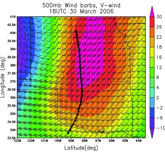
b) RHI plot of reectivity at same time as (a). Note: the storm is moving towards the radar, which is to the left in this image. c) Same as b) but for base velocity. Cross-sections in (b) and (c) are along line Aa in (a). 55 3.14 18 UTC 500 hPa v-wind component (shaded) and total wind (barbs) from

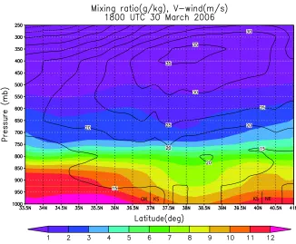
NARR data illustrating north/south variation in mid-level winds. This highlights a maximum in the southerly (line-parallel) wind component far-ther north in Kansas where the PS line formed, decreasing to the southwest where the supercells formed. . . 56 3.15 1800 UTC longitudinal cross-section taken at 98.5 W (just east of the

surface dryline) showing mixing ratio (shaded) and v-wind component (contoured) created from NARR data. . . 57 3.16 1856 UTC base reectivity data from Vance Air Force Base, Oklahoma

(14)

3.17 18 UTC 0-6 km wind shear vectors and magnitude (shaded) from NARR data illustrating north/south variation in vertical shear. This highlights both stronger shear magnitude to the south where the supercells formed as well as the larger across line component of the shear to the south vs. the larger along line component farther north. . . 59

4.1 Schematics of the various initiation mechanisms employed in the idealized model simulations. Note that while not shown, spacings of 0, 10, 20, 30 and 40 km were used between the bubbles within lines, and that both the line thermal and cold boxes contained random noise in order to help stimulate 3-dimensional structures. . . 83 4.2 Evolution of convection triggered using a single warm bubble in the LMN18

environment. Fields displayed are simulated radar reectivity at 3 km (shaded) and the edge of the surface cold pool, denoted by the -1 K surface potential temperature perturbation (heavy contour) at 90, 180, 270 and 360 minutes into the simulation. Note: only a portion of the domain is shown in order to highlight the storm details. . . 84 4.3 Simulated radar reectivity at 3 km, -1 K surface theta perturbation, and

3km wind vectors for LMN18 single bubble simulation at 270 minutes. . . 85 4.4 Simulated radar reectivity at 3 km and edge of surface cold pool denoted

(15)

4.5 Evolution of convection triggered using a single warm bubble in the TOP18nocap environment. Fields displayed are simulated radar reectivity at 3 km (shaded) and the edge of the surface cold pool, denoted by the -1 K sur-face potential temperature perturbation (heavy contour) at 90, 180, 270 and 360 minutes into the simulation. Note: only a portion of the domain is shown in order to highlight the storm details. . . 87 4.6 Simulated radar reectivity at 3 km, -1 K surface theta perturbation, and

3km wind vectors for TOP18 single bubble simulation at 270 minutes. . . 88 4.7 Simulated radar reectivity at 3 km and surface cold pool denoted by -1 K

potential temperature perturbation line for TOP18nocap environment: a) initiated with 200 km line thermal, 3 hours into the simulation. b) initiated with 3 warm bubbles spaced 20 km apart oriented northwest-southeast, 3 hours into the simulation. c) same as (b), but oriented north-south d) same as (b), but oriented southwest-northeast. Note: only a portion of the simulation domain is shown in order to focus on the details of the storm. 89 4.8 Plots of w (shaded, m/s), circulation wind vectors consisting of the u' and

w components of the wind and the 296 K theta contour representing the surface cold pool at 30 minutes for a) colliding outow boundary simula-tion, b) western outow boundary simulation c) eastern outow boundary simulation. Note: shading scale on (b) and (c) is 10% of that in (a) . . . 90 4.9 Cross-sections of simulated radar reectivity (dbz) circulation wind

(16)

4.10 Evolution of convection triggered using a single warm bubble in the TSF environment. Fields displayed are simulated radar reectivity at 3 km (shaded) and the edge of the surface cold pool, denoted by the -1 K surface potential temperature perturbation (heavy contour) at 90, 180, 270 and 360 minutes into the simulation. Note: only a portion of the domain is shown in order to highlight the storm details. . . 92 4.11 Simulated radar reectivity at 3 km and surface cold pool denoted by

-1 K potential temperature perturbation line for TSF environment: a) initiated with 5 bubbles spaced 20 km apart, 3 hours into the simulation. b) initiated with a 200 km line thermal, 3 hours into the simulation. c) same as (a) 6 hours into the simulation. d) same as (b) 6 hours into the simulation. Note: only a portion of the simulation domain is shown in order to focus on the details of the storm. . . 93 4.12 Simulated radar reectivity at 3 km and surface cold pool denoted by -1 K

potential temperature perturbation contour for environmental sensitivity runs at 180 minutes. a) LMN_TSF. b) LMN18_TOP18. c) TOP18nocap _TSF. d) TOP18nocap_LMN18. e) TSF_LMN18. f) TSF_TOP18. Note that the thermodynamic proles are constant horizontally, while the wind proles are constant vertically. . . 94 4.13 Simulated radar reectivity at 3 km and surface cold pool denoted by -1 K

(17)

4.14 Simulated radar reectivity at 3 km for a) LMN18 initiated with a 200 km line thermal, 60 minutes into the simulation, b) TOP18 initiated with a 200km line thermal, 60 minutes into the simulation, c) same as (a) at 120 minutes, and d) same as (b) at 120 minutes. . . 96 4.15 Plots of buoyancy acceleration (m/s) at 3 km 120 minutes into the

simu-lation for a) LMN18 and b) TOP18nocap_LMN runs described in gure 4.14. Note: That the domain and time of (a) and (b) correspond with gure 4.14c and d respectively. c) is a plot of the acceleration due to the vertical pressure gradient (shaded, m/s2_{) and circulation wind vectors}

con-sisting of the v and w wind components for the LMN18 simulation. The cross section is taken along the line Aa in gure 4.14. . . 97 4.16 Plots showing the change in 0-6 km vertical wind shear from the base state

(18)

(19)

List of Tables

(20)

Chapter 1 Introduction

1.1 Motivation

(21)

However, despite its importance in the formulation of an accurate severe weather forecast, convective mode remains dicult to anticipate and is an area of continuing research and focus (Kain et al. 2006). In line with past research, forecasters generally rely on analysis of vertical wind shear to determine the mode that storms will take (McNulty 1995; Edwards et al. 2002). This approach, however, can become complicated as dierent convective modes can occur within environments exhibiting similar wind proles (e.g. Bluestein and Jain 1985; Bluestein and Weisman 2000; Doswell and Evans 2003; Parker 2007a; b). It becomes complicated further in cases where two or more of these modes are present at the same time. One such event occurred on 30 March 2006 and is the focus of this study. This event featured isolated supercells, as well as linear MCSs with parallel and leading stratiform precipitation evolving simultaneously over eastern Kansas (Fig. 1.1). Accompanying the various modes, a variety of severe weather was observed as well. Large hail and tornadoes, including a long-track (25 km) F-2 in southeast Kansas were observed with several of the supercell storms (Fig. 1.2). Additionally, the PS line produced numerous hail reports, as well as damaging wind reports late in its evolution as it was transitioning toward the trailing stratiform (TS) mode. Given this wide range of severe weather, the 30 March 2006 case underscores the importance of improved understanding of multi-mode episodes while providing a well developed example of one such event.

(22)

in terms of the forecasting problem of not just determining the initial severe weather threat based on how storms will organize upon initiation, but then how that threat will evolve over time as storm organization evolves. Additionally, a broader goal of this study is to apply the ndings from this single multi-mode case to the larger problem of anticipating convective mode in similar moderate-high wind shear environments. Namely the goal is to identify various features that favor the development of each mode within the larger-scale moderate-high shear environment.

1.2 Structure of this thesis

(23)

PS

LS

Supercells

30 March 2006 19:52:58 UTC KICT 0.5 deg. Reflectivity N

5 15 25 35 45 55 65 75

10 20 30 40 50 60 70

dBZ

KICT

KTWX

(24)

0

0 0

1 1

1

2

03/30/2006 1800 UTC - 03/31/2006 0000 UTC Severe Reports

(25)

Chapter 2 Background

(26)

own mesoscale circulations a contiguous gust front, called a mesoscale convective system (MCS) (Maddox 1980). However, the convective cell forms the primary building block of organized convection.

The ultimate organization of a convective system, consisting of one or more convec-tive cells, is here referred to as the storm's organizational mode. Convecconvec-tive mode has been dened in many ways over a broad spectrum of scales. Some delineate between convective modes based on the dynamical structure of the cells that make up a given storm, essentially whether the system consists of ordinary, multi or supercells (Weisman and Klemp 1984). Some consider convective mode to refer to the meso-beta scale storm characteristics dealing with storm organization and appearance on radar, such as whether storms appear isolated, clustered (e.g. a multicell cluster) or linear in nature (Kain et al. 2006). Still others make more precise divisions among subsets of a larger group of storms, such as mesoscale convective systems with trailing, linear, and parallel stratiform precip-itation (Parker and Johnson 2000). And yet others determine variations in mode based on storm formation, such as the dierent means for isolated severe storm development along the dryline outlined by Bluestein and Parker (1993) or dierent modes of mesoscale convective line development discussed by Bluestein and Jain (1985).

(27)

linear modes can each be associated with dierent types of severe weather (as discussed in Chapter 1). In order to best introduce the scientic problem at hand, this section will rst look at the individual modes of interest in detail, then discuss the dierences in environment and dynamics that result in said modes.

2.1 Convective Modes in Detail

2.1.1 Supercells

(28)

severe weather events (e.g. hail > 5 cm, winds > 33 m/s, tornadoes > F2) do tend to be associated with these storms resulting in an increased severe weather threat associated with supercells (Doswell 2001).

2.1.2 Squall Lines

While the term squall line has historically been used to refer to a variety of meteo-rological phenomena, with regard to convective storms, squall line refers a to linearly oriented MCS (Bluestein and Jain 1985). More specically, squall lines consist of multi-ple, interacting, convective cells that share a common leading edge and appear as a line or arc with no breaks in precipitation between the cells (Doswell 2001). These cells can range from short-lived ordinary cells, which would require the frequent triggering of new cells to sustain the system, to organized supercells which would result in a squall line of long-lived individual cellular elements (Bluestein and Jain 1985). However, many squall lines are made up of elements that behave similarly to multicell storms, with periodic regeneration of new cells as old ones decay (Houze et al. 1989). In addition to cellular convection, there are also cases wherein a squall line consists of a swath of contiguous lifting, referred to as slabular lifting (James et al. 2005). This type of lifting tends to occur in conditions wherein a strong cold pool is present to create a broad area of lift.

(29)

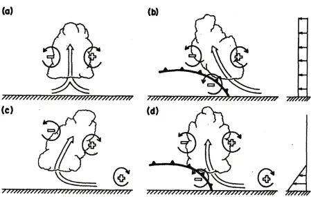
and orientation of environmental wind shear does play a role in the organization of cells within the squall line (i.e. whether the line contains ordinary cells or supercells) it also also plays an important role in squall line longevity (Rotunno et al. 1988). In a long-lived squall line, low level wind shear balances the cold pool circulation generated by the gust front as the cold pool spreads beneath the storm. Without shear the gust front would just move away from the storm, resulting in no new convective development and a short-lived storm. However, with low level wind shear to oppose this cold pool motion, the gust front remains close to the storm and a shear-induced circulation balances the cold pool circulation resulting in new convective development and a long-lived storm. In the optimal case where the shear and cold pool balance each other, this will lead to an upright updraft, and a strong, long-lived storm (Figure 2.4) (Rotunno et al. 1988).

In general, squall line formation necessitates some means to force linear organization. Such organization can come from synoptic scale features such as fronts and drylines, wherein a broad region of forcing is present. Oftentimes convection will be initiated along one of these boundaries in isolated pockets and then grow along the line as the initial cells grow in size and new ones form between them (Bluestein and Jain (1985)'s broken line). In other cases, an isolated cell or group of cells along a boundary will evolve into a line through repeated new cell development occurring upstream (with respect to cell motion) along the line that then merges with the old cell (Bluestein and Jain (1985)'s backbuilding). Squall lines can also form in the absence of strong synoptic forcing, such as from the mergers of two or more isolated cells, such as supercells (e.g. Bluestein and Weisman 2000; Finley et al. 2001). In these cases the merger will often result in the strengthening of surface outow, leading to development of new convection in a more linear organization along the outow boundary.

(30)

be maintained through consistent lifting along the leading edge of the gust front and the generation of new cells as older cells mature and decay while moving rearward, similar to the multicell regeneration process (Houze et al. 1989). As this process continues it will lead to a region of intense convective precipitation, along with a broad area of weaker stratiform precipitation. Figure 2.5 shows the classic trailing stratiform (TS) structure that is found in many squall lines. Intense convection is found at the leading edge of the line in the region of strongest ascent along the gust front with a broad region of stratiform precipitation behind the line due to to hydrometeors being advected rearward over the cold pool by an ascending front to rear ow (Houze et al. 1989). Since this front to rear ow is favored in systems with strong cold pools (Rotunno et al. 1988), it makes sense that linear MCSs with strong cold pools favor, and ultimately evolve towards, the TS structure. While the trailing stratiform structure tends to be the most common type of squall line, two other modes have been identied based on the structure of their stratiform regions; the leading stratiform linear MCS, wherein the stratiform region precedes the convective region of the line, and the parallel stratiform linear MCS, wherein the stratiform region is oriented parallel to the convective line (Figure 2.6) (Parker and Johnson 2000).

2.1.2.1 Convective Lines With Leading Stratiform Precipitation

(31)

types of LS systems have been observed in nature: rear-fed LS and front-fed LS. The key dierence between the two types is the source of inow, with rear-fed systems being sustained by inow from behind the line (Pettet and Johnson 2003) while front-fed LS systems are sustained by inow from ahead of the line that passes through the stratiform region (Parker and Johnson 2004c). Given that the front fed systems are more numerous in nature, they have received more attention in the literature, and the majority of the knowledge regarding LS systems relates to this type.

LS MCSs can largely be approximated as 2-D entities as evidenced by Parker and Johnson (2004c) (Figure 2.7). A key dynamical feature of these systems is an overturning updraft wherein inowing air enters from ahead of the line, ascends through the updraft and then is accelerated downshear ahead of the line (Parker and Johnson 2004a). This acceleration is due to transient accelerations generated by buoyancy, as well as linear and non-linear pressure elds (Parker and Johnson 2004a). The leading precipitation eventually causes a transition to the trailing stratiform (TS) structure, as buoyancy-induced pressure perturbations lead to a decrease in vertical wind shear in the pre-line region. This, combined with a strengthening cold pool, result in a rearward sloping of the updraft and eventual transition to a TS system (Parker and Johnson 2004b). This evolution from LS to TS occurs a majority of the time (Parker and Johnson 2004c), especially for long-lived cases and was indeed seen within some of the LS simulations performed in this study, namely those initiated with a signicantly colder initial cold box.

2.1.2.2 Convective Lines With Parallel Stratiform Precipitation

(32)

(33)

shear may permit three distinguishable primary structures. This makes it less surprising that all three modes were observed on 30 March 2006, however it does not answer the question of how all three managed to be simultaneously present in close proximity to each other. To continue to get to the root of this problem, some of the mechanisms that drive convective mode in more general terms will now be reviewed.

2.2 Delineation Between Modes

(34)

nature of the ow elds.

This rst study oered a great deal of insight into some of the environmental factors that eect convective storm type, however the authors admitted that there were some shortcomings, namely that the two dimensional shear prole failed to account for direc-tional wind shear, which at the time was suggested to play an important role in storm structure, especially for supercell storms. To address this, the authors did another study in 1984, this time using a three dimensional wind eld which allowed for directionally varying wind shear. When directional shear was added to the model, the authors still found an increase in organization with increasing shear. They observed a spectrum of storms from short-lived isolated convection to multicells to supercells as shears progressed from low to moderate to high. They did nd, though, that the storm structures varied somewhat compared to the previous study. For instance, with a clockwise turning hodo-graph supercell development was favored on the right ank of storms, while the left ank tended towards more of a multicell development. In moderate shears these two modes evolved together, which the authors pointed out is similar to what is sometimes observed in nature where a supercell will be present at the southern end of a squall line (Weisman and Klemp 1984).

(35)

ank storms consist of multiple short-lived updrafts that generally move with the mean wind. These updrafts are initially forced by a surface gust front, and 60-70% of their strength is attributed to buoyancy forcing. Mid-level vorticity maxima are found with these storms as well, but they do not correlate strongly with the updraft locations. Given these dierences, the authors suggest two main modes of storms, multicells and supercells, based on the dynamical dierences described above. Larger organized convective systems such as squall lines are then seen as consisting of a combination of these two types. Since these features largely depend on vertical wind shear and buoyancy, the authors suggest that these factors continue to be the keys in determining convective mode.

(36)

with rather surprising results.

(37)

While it is clear from the above studies that shear and buoyancy play an important role in determining convective mode, the presence of linear boundaries such as outow boundaries and dry lines can be important as well, especially when considered along with wind shear1_{. This is not a new idea, having been introduced by Bluestein and}

Jain (1985) wherein the authors speculated as to why they observed both supercells and backbuilding squall lines forming in similar environments, and in similar proximity to surface boundaries. The authors hypothesized that the orientation of the vertical shear with respect to the boundary may be important, however their limited investigations using observed data met with little success. Fifteen years later, Bluestein and Weisman (2000) examined the eect of varying the orientation of wind shear vectors with respect to a line of forcing (in their case a dryline) on numerically simulated supercells. The study used idealized model simulations that included a pseudo dryline as well as a line of supercells initiated using warm bubbles, to which the authors introduced wind shear that was perpendicular, oblique (45◦_{), and parallel to the line. They found that for}

shear perpendicular to the line, the simulation generated a squall line with right and left moving supercells at either end. For shear oblique to the line, the result was a line of isolated (i.e. not interacting) right moving supercells. Finally for shear parallel to the line, the authors found a right moving supercell at the downshear end of the line, along with a left moving supercell that has some multicell characteristics, and most of the rest of the cells along the line devolved to ordinary cells after interacting with their neighbors (Bluestein and Weisman 2000). This suggests that when a linear forcing mechanism such as a dryline is present, just the mere presence of shear is not enough to determine the mode, but rather how that shear is oriented with respect to the line matters as well.

1_{In this sense boundary refers to mesoscale boundaries such as drylines or outow boundaries. For}

(38)

In the simulations, curved hodographs indicative of supercells were used in every case, however, the results show that depending on the shear's orientation to the simulated dryline, dierent modes can result despite the presence of a supercell environment.

(39)

role in determining convective mode by themselves.

In addition to their discussion of the importance of shear relative to a boundary, Bluestein and Weisman (2000) also discussed the importance of cell interactions in deter-mining convective mode. For most cases within their simulations, when a cell encountered another cell or its outow, it tended to lose its supercellular characteristics and multi-ple interactions often led to the development of a squall line. Simulations by Finley et al. (2001) demonstrated the role that cell mergers can play in the transition of a high-precipitation supercell to a bow echo. In the simulated event, the merger of a pair of supercells led to increased precipitation resulting in cold pool intensication and the transition to a bow echo structure. Thus cell interactions can have a signicant eect on convective mode when multiple storms are present.

(40)

these two modes.

(41)

(42)

(43)

(44)

Figure 2.4: The eects of wind shear and cold pool induced circulations on a squall line updraft. a) No shear or cold pool results in a vertical updraft. b) No shear with a cold pool results in an updraft that tilts rearward over the cold pool. c) Shear with no cold pool results in an updraft that tilts forward. d) Shear and cold pool in optimal balance results in vertical updraft. (from Rotunno et al. 1988).

(45)

100 km

Linear MCS archetypes

a.

b.

c.

Trailing stratiform

Leading stratiform

Parallel stratiform

Initiation

Development

Maturity

TS

LS

PS

(46)

weakly ascending front-to-rear inflow stream mean overturning updraft

outflow boundary/ gust front

region of intense convection

"up-down" trajectories

quasi-horizontal rear-to-front airstream

(47)

e v it a l e r -m r o t s e n il -g n o l a li v n a n i w o lf l o o p d l o c r a e r -o t -t n o r f w o l f n i e v i t a l e r -m r o t s i f o n o i g e r n o i t c e v n o c e s n e t n / y r a d n u o b w o lf t u o t n o rf t s u g

~ 50 k m horiz. ~ 1 0 k m v er t. leading trailing left right

(48)

Chapter 3 Observational Case Study

The aforementioned case of 30 March 2006 will serve as the basis for the observational case study and subsequent numerical simulations, as it is a prime example of a multi-modal event, with supercells, an LS MCS and a PS MCS present over a localized region (Fig.1.1). The data and methods used in the case study will be discussed rst, followed by a discussion of the results of this portion of the study.

3.1 Case Study Methodology

(49)

and Doppler velocity observations covering the scope of the event (Fig. 3.1). Finally, the radiosonde wind proles were supplemented by hourly observations from regional NOAA Wind Proler sites (Fig. 3.1).

In addition to these actual observations from the day in question, the North Amer-ican Regional Reanalysis (NARR, Mesinger et al. 2006) was used to supplement the observations because of its enhanced coverage and resolution. This resulted in a more complete picture of the event, especially in the vertical, and allowed for cross-sectional analyses of important features such as the surface dryline. In order to ensure accuracy, the NARR data were compared to available observations at both 1200 and 1800 UTC on 30 March as well as 0000 UTC on 31 March, and were found to be representative of regional soundings and surface observations. This collection of observations and NARR data was analyzed both objectively and subjectively to gain a detailed picture of the storms and their environments throughout the duration of the event.

(50)

as a somewhat unique example of a multi-mode event. Dial and Racy (2004) found, in a study of 37 cases, that mixed-mode events (dened as consisting of linear and isolated modes) occurred approximately 19% of the time for their parameter space. This suggests that while not an everyday occurrence, these multi-mode events occur often enough to be of concern to forecasters, especially given their wide-ranging severe weather threat.

3.2 Case Study Results

The case of 30 March 2006 included three distinct modes of convection: an MCS with parallel stratiform precipitation in central Kansas, an MCS with leading stratiform precipitation in far eastern Kansas, and a group of isolated supercells in east central Kansas (Fig. 1.1). All were present at the same time and within an area of less than 400 km x 500 km.

3.2.1 Background environment

Key features of the pre-storm synoptic environment are summarized in Fig. 3.2 . This environment was characterized by a large amplitude, diuent, middle and upper level trough over the Rocky Mountains evident at 500 hPa (Fig. 3.2b). A 35 m/s jet curved around the base of this trough from the west coast into the southern plains, with an embedded 45 m/s jet streak over New Mexico and Arizona (Fig. 3.2a). At lower levels, an 850 hPa 25 m/s southwesterly low level jet was transporting warm moist air into Oklahoma and Kansas (Fig. 3.2c). The key surface feature for this event was a dryline that extended from a low pressure center in north central Kansas southward into northern Texas (Fig.3.3). Ahead of this dryline, temperatures had warmed into the 18-20◦_{C range}

(51)

into south-central Kansas. West of the dryline temperatures were approximately 5◦_C

higher while dew points were signicantly lower, with a narrow axis of very dry air extending from southwest Kansas through central New Mexico. The 1800 UTC upper air soundings from around the region indicated a moderately unstable (CAPE of 1000-2000 J/kg), weakly capped environment to the east of the dryline (Fig.3.4) characterized by moderate to strong vertical wind shear (Fig.3.5).

Taken as a whole, these features indicate an environment primed for convective storms. Synoptic-scale sources of lift were present in the form of the upper level trough and jet streak, as well as large scale low level warm advection. The surface dryline pro-vided a localized focus for lifting in the boundary layer. CAPE values in the 1000-2000 J/kg range suggested that storms would have ample instability to fuel their development, while the moderate (15-20 m/s) to high (> 20 m/s) wind shear suggested supercells or squall lines were possible (Rasmussen and Blanchard 1998; Evans and Doswell 2001). Thus the background environment for this case was very favorable for organized, strong convective storms. In such a case, an operational forecaster might be led to expect one predominant convective mode to emerge; but instead several unique and long-lasting storm types occurred.

3.2.2 Radar Analysis

(52)

UTC. During the course of this time period the storms involved aected central and east-ern Kansas, most of northeast-ern Oklahoma and parts of westeast-ern Missouri. Each convective mode's formation and evolution will now be described in turn.

The storms that would evolve into the isolated supercells on 30 March 2006 event were initiated along and just ahead of a surface dryline in western Oklahoma at approximately 1630 UTC (Fig. 3.7). While the initial storms consisted of both isolated and broken linear structures, they quickly moved northeastward o of the dryline, becoming increasingly isolated in nature while intensifying and developing supercellular characteristics (Fig. 3.6a). By 1845 UTC these had become a collection of isolated storms oriented northeast to southwest from eastern Kansas into central Oklahoma, with well-developed mesocyclones and hook-echo structures evident (Fig. 3.8a,b). A range-height indicator (RHI) scan through one these storms reveals a bounded weak echo region (BWER), further indicating the supercell mode. Additionally, these storms produced numerous reports of severe hail greater than 1 in diameter, as well as several tornado reports (Fig. 1.2). The isolated supercellular organization of these storms remained until their eventual dissipation in eastern Kansas and Oklahoma.

(53)

central Kansas, and a region of stratiform precipitation located at the northern end of this line (Fig. 3.10a). Range-Height Indicator (RHI) plots taken in both the across and along-line directions further illustrate the PS structure, indicating little stratiform precipitation ahead of or behind the line (Fig. 3.10c), and substantial stratiform pre-cipitation north of the strongest convection, parallel to the convective line (Fig. 3.10b). This MCS was fairly similar in structure to the 2 May 1997 PS MCS analyzed by Parker (2007a), including a radar-indicated ne line structure extending south of the line (Fig. 3.10a). In the present case, this appears to be an indication of the surface dryline, based on surface observations taken as the feature passed.

The PS system progressed eastward across Kansas, remaining just ahead of this sur-face dryline, and eventually evolved into a linear MCS with trailing stratiform precipita-tion (TS) by 2100 UTC (Fig. 3.11) as is often observed with this convective mode (Parker and Johnson 2000; Parker 2007a). After the transition to the TS mode, the MCS began to weaken as it crossed northeastern Kansas and southeastern Nebraska, losing most of its organization by approximately 2330 UTC. During its evolution, this MCS generated severe hail, with reports of greater than 2 diameter hailstones (Fig. 1.2). These hail reports came rst from the initial cells near the northern edge of the line, which exhib-ited higher reectivities, and continued to contain weak mesocyclones throughout the rst 1-2 hours of PS evolution, although scattered severe hail was also reported along the remainder of the convective line throughout the course of the event. Additionally, the PS line was not associated with any severe wind reports until after it had transitioned to the TS mode in northeastern Kansas.

(54)

the dryline, as was the case with the supercells and PS line, these storms appear to have been forced by a collision between two outow boundaries. Surface observations in this area were sparse, however earlier observations in the vicinity of the supercells recorded temperature drops of 6◦_{C within the storms and 2-3}◦_{C near their periphery, suggesting}

at least some weak outow from these storms. Observations to the east where the LS line formed also show slightly (1◦_{C) cooler temperatures suggesting an area of weak outow}

that resulted from the passage of earlier convection (visible near KTWX in gure 3.6a, b). The strongest evidence of this outow collision, though, can be seen in the radar data which shows two ne lines, indicative of boundaries, that appeared to merge as this line developed (Fig. 3.12). Following the merger, a squall line rapidly back built to the south, and eventually produced leading stratiform precipitation (Fig. 3.13a). An RHI plot, taken in the across-line direction at 2103 UTC shows two key elements of the front-fed LS structure (Parker and Johnson 2004c); the leading stratiform region in the reectivity eld (Fig. 3.13b), as well as the characteristic pre-line structure of low level ow toward the convective line, with mid and upper level ow away from the convective line (Fig. 3.13c). Unlike the supercells and PS MCS, the LS line produced very little in the way of severe weather, with only some very widely scattered reports of severe hail during its evolution. The storm maintained its leading stratiform structure as it moved east into Missouri, where it eventually began dissipating by 2230 UTC.

3.2.3 Environmental and Initiation Variations

(55)

to the environment in eastern Kansas where the LS line formed, and eventually where all three modes were present. Finally, some dierences in storm initiation mechanism and their possible implications with regards to convective mode will be discussed as well.

3.2.3.1 Mid-Level Winds

One important dierence between the supercell and PS environments is the variation in the direction of the mid-level winds in relation to the dryline due to the location of the upper level trough. To the south, across Oklahoma, winds were more westerly above the dryline whereas to the north, they were more southerly and more nearly parallel to the dryline (Fig. 3.14). This can also be seen in gure 3.15 as a stronger v-component of the 500 hPa environmental wind is evident farther to the north, suggesting a larger dryline-parallel component of the wind in this region. A larger along-line component of the mid-level ow would allow the storms to remain close to the boundary and its associated linear forcing, likely favoring more linear evolution like the PS system in central Kansas. A larger across-line component would likely cause cells to move o the dryline and away from the linear forcing, favoring more isolated storms such as the supercells in western Oklahoma. Figure 3.16 illustrates that this was indeed the case. By around 1900 UTC, the supercells had moved well o the dryline, while the PS line was anchored just ahead of it.

Boundary-relative ow aloft also plays a role in the interactions among neighbor-ing convective cells insofar as it relates to the direction of the deep layer shear vector. Bluestein and Weisman (2000) determined that for shear vectors oriented 45◦ _{from a}

(56)

a 45◦ _{angle with the dryline (Fig. 3.17), and the initial cells and broken lines moved}

o of the dryline and evolved into isolated supercells. In contrast, an environment with a larger along-line component tends to favor linear modes as along-line shear tends to result in cell mergers, which have been shown to be detrimental to long-lived isolated structures and instead favor linear modes (Bluestein and Weisman 2000). Furthermore, this can lead to the seeding of hydrometers into downstream cells aloft expediting cold pool development, and leading to a strong, broad cold pool favoring a linear mode (e.g. Dial and Racy, 2004; Parker, 2007a). Such an environment, containing along-line shear was present farther north along the dryline where the PS line developed (Fig. 3.17). While there were no observations of ne enough scale to determine specic hydrometeor motions, radar animations do indicate the presence of cell collisions during the develop-mental stages of the PS line. As well, given the along-line hydrometeor transport that is necessary for the formation of a region of parallel stratiform precipitation it is also likely that seeding occurred, much as was seen in the PS simulations of Parker (2007a; b).

3.2.3.2 Dry Air Aloft

(57)

been present ahead of the dryline in west-central Kansas 6 hours earlier.

The presence of dry air aloft in the region where the squall line formed is signicant, as dry air can enhance cold pool development due to evaporational cooling. This would favor the development of linear modes as stronger cold pools tend to spread and interact, resulting in a broad region of linear lifting along the leading edge of the cold pool. Some evidence of this stronger cold pool development in the region of the PS line (relative to that seen with the supercells to the south) was evident on 30 March 2006. Just after 1900 UTC the observations from Concordia and Salina Kansas, in the vicinity of the PS line, both registered temperature decreases of approximately 6◦_{C, with the colder}

temperatures remaining in place for close to an hour. Salina also recorded a 2 hPa increase in pressure during this time. Observations from Newton, Kansas taken as one of the supercells passed near the observing station also show a 6◦_{C temperature decrease,}

however the areal extent of this cold pool was much smaller, as nearby stations in Wichita recorded temperature decreases of only 2-3◦_{C, and these were of shorter duration than}

the observed decreases in Salina and Concordia. Furthermore, there were no discernible pressure changes with the passage of the supercell, suggesting that while the precipitation had a cooling eect on the lower levels, the cold pool was not as strong as that seen farther north with the PS line. These observations would suggest that the lack of dry air aloft farther south resulted in weaker, smaller cold pools, aiding in the maintenance of an isolated mode.

3.2.3.3 Initiation Mechanisms

(58)

the LS line developed along an apparent outow collision, suggesting two distinct forcing mechanisms. Looking closer at the supercells and PS line, further variations emerge, as the supercells were initiated as more widely spaced isolated and broken linear entities while the PS line developed from several closely spaced cells. Orientation of these initial cells is important to note as well, as the initial storms that led to the supercells were initially oriented in a more southwest-northeast line, while those that developed the PS line were in a more north-south line. These variations in initial cell orientation may have been an important part of the 30 March event, as Bluestein and Weisman (2000) demonstrated that cell orientation relative to the vertical wind shear vector can have important eects on storm mode. These dierences in cell orientation will be investigated further using the idealized model simulations discussed in chapter 4.

3.2.3.4 Moderate Shear Environment

A nal environmental variation that likely played a role in the evolution of the 30 March 2006 event was the presence of a region of weaker vertical wind shear across eastern Kansas where the LS line formed. The environments that spawned the supercells and PS MCS were both characterized by high 0-6 km wind shears of approximately 25 m/s, which is understandable given that both modes are favored in high-shear environments (Parker 2007a). However, the environment over eastern Kansas, characterized by the 18 UTC Topeka radiosonde observation, contained a more moderate 0-6 km wind shear of 18 m/s (Fig. 3.5b). This suggests an environment that could sustain both multicell and supercell storms (as documented in the simulations of Weisman and Klemp 1984), playing an important part in the evolution of the 30 March event in two ways.

(59)

in shape to that from Lamont (Fig. 3.5a,b), however, the weaker 0-6 km wind shear in Topeka made it less favorable for supercells. This environment was combined with the strong linear forcing of the colliding outow boundaries, favoring linear modes even more. Outows are typically associated with 'slabular,' or layer-like, lifting (James et al. 2005), so the collision of outows is likely to result in a strong preference for slabular lifting (Fig. 3.12), as opposed to the more isolated cellular lifting that was seen along the dryline, where the supercells and PS line formed (Fig. 3.6a). Given that the MCS that developed was oriented largely north-south, the environmental shear vectors ended up being directed largely across-line, thus ruling out the development of the PS mode. And while the shear was less than seen in the supercell and PS environments, it was still strong enough to favor the LS precipitation structure (Parker and Johnson 2004c).

(60)

of convection. It is hypothesized that this was made possible by this moderate shear environment containing enough wind shear to support the on-going supercells, while not containing so much shear that the linear MCSs evolved into more isolated or supercellular structures.

(61)

(62)

KTOP

KDDC

KSGF KLMN

KOUN KAMA

KFWD KOAX

KTWX

KICT

KVNX

KEAX

HVLK1

HBRK1

LMNO2 FBYN1

LTHM7

NDSK1 RWDN1

KSLN

Upper AirSites

NOAA Wind Profiler Sites WSR-88D Radar Sites ASOS Sites

Legend

(63)

(a) (b)

(c)

(64)

996

1000 1004

1008

1012

1008

L

(65)

SBCAPE: 1738 J/kg SBCIN: 0J/kg MLCAPE: 1113 J/kg MLCIN: -8 J/kg

(66)

0 10 20 30 40 50 0 10 20 30 40 50

0 10 20 30 40 50

0-12 km hodograph 18 UTC 30 March 2006 Fairbury, Nebraska

0 3 6 9 12 0 3 6 9 12 0-12 km hodograph

18 UTC 30 March 2006 Lamont, Oklahoma

0

3 6

9

12

0-12 km hodograph 18 UTC 30 March 2006 Topeka, Kansas

0-6 km shear vector magnitude: 25 m/s

0-6 km shear vector magnitude: 18 m/s

(a) (b)

(c)

(67)

5 15 25 35 45 55 65 75 10 20 30 40 50 60 70 80 dBZ

KICT 0.5 deg. Reflectivity 30 March 2006 18:02:10 UTC

KICT KTWX (a) 5 15 25 35 45 55 65 75 10 20 30 40 50 60 70 80 dBZ

KICT KTWX (b) 5 15 25 35 45 55 65 75 10 20 30 40 50 60 70 80 dBZ

KICT KTWX (c) 5 15 25 35 45 55 65 75 10 20 30 40 50 60 70 80 dBZ

KTWX 0.5 deg. Reflectivity 30 March 2006 21:59:49 UTC

KICT

KTWX

(d)

(68)

KVNX

KICT 30 March 2006 16:58:00 UTC KVNX 0.5 deg. Reflectivity

5 15 25 35 45 55 65 75

10 20 30 40 50 60 70 80 dBZ

(69)

0 6 12 18 24 30 36 42 48 54 60 66 72 78 84 90 3 6 9 12 15

Distance From Radar (km)

A

lt

it

ude (k

m)

KICT Range Height Indicator Base Reflectivity 30 March 2006 19:10:47 UTC

0 40 45 50 55 60 65 70 75 35 30 25 20 15 10 5 dBZ 80 A a (c) (a)

30 March 2006 19:10:47 UTC KICT 0.5 deg. Reflectivity

KICT 5 15 25 35 45 55 65 75 10 20 30 40 50 60 70 80 dBZ A a (b) -45 -30 -15 0 15 30 45

30 March 2006 19:12:07 UTC KICT 1.3 deg. Storm Relative Velocity

-60 60 KTS

(70)

5 15 25 35 45 55 65 75

10 20 30 40 50 60 70 80

dBZ 30 March 2006 17:53:43 UTC KICT 0.5 deg. Reflectivity

(71)

A a

0 35 70 105 140 175 210 245 3

6 9 12 15

A

lt

it

ude (k

m)

KICT Range Height Indicator Base Reflectivity 30 March 2006 19:48:45 UTC

0

a A

B b

5 15 25 35 45 55 65 75 10 20 30 40 50 60 70 80 dBZ KICT KTWX B b (a) (c) (b) A a 0 20 40 60 80 100 120

140 130 110 90 70 50 30

150 10

12

A ltitu de ( k m)

KTWX Range Height Indicator Base Reflectivity 30 March 2006 19:47:06 UTC

0 40 45 50 55 60 65 70 75 35 30 25 20 15 10 5 dBZ 80 9 6 3 40 50 55 60 65 70 75 35 30 25 20 15 10 5 dBZ 80 45

(72)

KTWX

5 15 25 35 45 55 65 75

10 20 30 40 50 60 70 80

dBZ 30 March 2006 22:04:06 UTC KTWX 0.5 deg. Reflectivity

(73)

30 March 2006 18:53:52 UTC KICT 0.5 deg. Reflectivity 5 15 25 35 45 55 65 75 10 20 30 40 50 60 70 80 dBZ KICT (a)

KICT 5 15 25 35 45 55 65 75 10 20 30 40 50 60 70 80 dBZ (b)

KICT 5 15 25 35 45 55 65 75 10 20 30 40 50 60 70 80 dBZ (c)

KICT 5 15 25 35 45 55 65 75 10 20 30 40 50 60 70 80 dBZ (d)

(74)

3 6 9 12 15

A lti tu d e (k m) 0 Storm Motion 0 5 10 20 30 40 50 60

70 65 55 45 35 25 15

75

Distance From Radar (km)40 30 20 10 5 0 50

60

70 65 55 45 35 25 15

75

Storm MotionStorm Motion

3 6 9 12 15 A lti tu d e (k m) 0 0 10 20 30 40 50 60 70 -10 -20 -30 -40 -50 -60 -70

KTS _{KEAX Range Height Indicator Base Velocity}

30 March 2006 21:03:59 UTC

30 March 2006 21:03:59 UTC KEAX 0.5 deg. Reflectivity

KEAX KTWX A a 5 15 25 35 45 55 65 75 10 20 30 40 50 60 70 80 dBZ (c) A a (b) (a) 40 45 50 55 60 65 70 75 35 30 25 20 15 10 5 dBZ

80 KEAX Range Height Indicator Base Reflectivity

30 March 2006 21:03:59 UTC

A a

(75)

(76)

NE KS KS

OK

(77)

KVNX

KICT

5 15 25 35 45 55 65 75

10 20 30 40 50 60 70 80 dBZ

30 March 2006 18:56:48 UTC KVNX 0.5 deg. Reflectivity

PS

Supercells

(78)

(79)

Chapter 4 Model Simulations

(80)

environmental shear will favor isolated modes whereas shear parallel or perpendicular to the initial cells will favor linear modes, as suggested by the observations, and described by Bluestein and Weisman (2000). In order to test these hypotheses, idealized simulations were used to try to isolate the eects of the environment vs. the initiation mechanism on convective mode. Additionally, the possibility of storms altering their local environment is examined as well. Idealized numerical simulations were chosen because within controlled simulations one can isolate processes in ways that are not possible in nature. A simulation of the actual case was attempted as well, as a means to bridge the gap between the observed case and the idealized simulations.

4.1 Idealized Simulations

4.1.1 Methods and Conguration

(81)

parameterize cloud and precipitation microphysics. Sub-gridscale turbulence was param-eterized using a 1.5 order turbulent kinetic energy (TKE) closure. Coriolis accelerations, were not included in the model given the short integration time, a common practice in idealized studies (e.g. Rotunno et al. 1988; Bluestein and Weisman 2000; James et al. 2005; Parker 2007a,b). Furthermore, simulations by Parker (2007b) demonstrated that the overall convective mode was not sensitive to variations in Coriolis during a 6-hour simulation. To further simplify the simulations, surface uxes and radiative eects were not included in the model. The simulations used Rayleigh damping over a layer of 5 km at the model top, and open lateral boundary conditions unless otherwise noted. The ini-tial conditions were homogeneous, with articial perturbations added to initiate storms as will be discussed shortly. For these simulations, the pre-packaged em_quarter_ss experiment was utilized as the initial source code and then modied to produce the setup described herein.

(82)

these colder temperature would appear to be at odds with observations that suggested the coldest air in the supercell cold pools was very limited. Because the constant grid spacing better replicated the variety of modes observed, which were focus of this study, this setup was used for the idealized simulations.

(83)

(84)

signicant noise at the inow (western) lateral boundary causing the model to become unstable. By stretching the domain in the x-direction and making the lateral boundaries periodic, this problem was eradicated without detriment to the storms being simulated.

4.1.2 Environmental Control Simulations and Initial

Perturba-tion Sensitivities

To establish control runs, idealized simulations were performed using each of the initial soundings and a single warm bubble perturbation to initiate convection. The single-bubble simulations established the relationship between a given environment and its predominant convective mode while at the same time providing benchmarks with which to compare further sensitivity tests. Following these initial runs, the initial perturbation was varied to examine the sensitivity of convective mode to forcing mechanism within each environment.

The rst experiment used the LMN18 sounding characterized by a moderate amount of CAPE and strong wind shear. The single bubble quickly triggered an isolated storm (Fig. 4.2a) that began evolving toward a supercell by 3 hours into the simulation (Fig. 4.2b). By 4.5 hours, the storm had developed into a mature supercell (Fig. 4.2c) charac-terized by a mid-level mesocyclone, along with hook echo and bounded weak echo region (BWER) features in the simulated reectivity elds (Fig. 4.3). This storm remained a supercell for the duration of the 6-hour simulation (Fig. 4.2d).

(85)

were expected to develop in some of the other simulations, especially with the line thermal and cold box triggers. For these simulations, the initial storms that formed were indeed linear, however these linear structures rapidly devolved into individual cells, with the southernmost cell dominating and becoming a long-lived supercell (Fig. 4.4 a, b). Similar results were seen from the lines of warm bubbles, wherein convection began as a line of isolated cells, with the northern cells weakening with time and the southernmost cell dominating and evolving into a long-lived supercell (Fig. 4.4c, d). This evolution towards increasingly supercellular structures is similar to what was seen in Oklahoma during the 30 March case. The initial cells and broken line segments became more organized and supercellular with time as they evolved across the region. This suggests that within the high CAPE, strongly sheared environment seen in western Oklahoma on 30 March 2006, environmental factors played a larger role than initiation mechanism in selection of convective mode. The environment strongly favored supercells, and that was the ultimate mode that evolved irregardless of how the simulated storms were initiated.

The second environment represented eastern Kansas, where the LS system was ob-served and was characterized by the 18 UTC TOP18nocap sounding. This region was very similar to the supercell environment, except that the 0-6 km bulk shear vector magnitude was approximately 6-8 m/s weaker. The single-bubble simulation resulted in a splitting supercell (Fig. 4.5a) whose right-moving entity displayed supercell char-acteristics (Fig. 4.3) while continuing to periodically split, with the left-moving storms evolving as multicells (Fig. 4.5b) . Eventually several of these smaller multicells merged and formed an LS squall line to the north of the supercell (Fig. 4.5c). These two modes continued to evolve together through the remainder of the simulation, with the supercell beginning to merge into the southern end of the line by six hours (Fig. 4.5d).

(86)

mech-anism using the TOP18nocap and TOP18 soundings using the same set of initiation mechanisms as was used with the LMN18 sounding. For these simulations, the ulti-mate mode observed was seen to be sensitive to initiation mechanism, mainly when the orientation of the initial cells was manipulated. The lines of 5-bubbles1_{, cold box, line}

thermal and lines of 3-bubbles oriented northwest-southeast all behaved very similarly to the control run, as illustrated in gures 4.7a and 4.7b. The only dierence observed with these runs was a larger areal extent of the convection, owing to the larger size of the initial perturbation. The gross modal characteristics, though remained the same. A more signicant sensitivity was seen from both the line of 3 bubbles oriented north to south (hereafter TOP18_3bubNS) and the line of 3 bubbles oriented southwest to north-east (hereafter TOP18_3bubSwNe). The TOP18_3bubNS simulation behaved similarly to the control run through about 4 hours, but then the supercell rapidly merged with the south end of the squall line and the system subsequently evolved towards the TS precipitation structure (Fig. 4.7c). The more rapid merger was due to the supercell being overtaken by the southern edge of the squall line's cold pool. It is of note that in this case, the areal extent of the squall line was more compact, and the embedded echos appeared more intense than seen during the evolution of the control simulation. Indeed, by 6 hours, the areal extent of the line in this simulation is much smaller (Fig. 4.7c) than seen in the control simulation or any of the simulations that behaved like the control simulation (e.g. Fig. 4.7a and b). This more compact area of intense convection could have lead to the development of a stronger cold pool, which would account for both the faster merger and the evolution toward TS.

The TOP18_3bubSwNe simulation also evolved dierently than the control

simula-1_{In every case, the same behavior was seen from a given orientation of the lines of warm bubbles}

(87)

tion, as the three initial cells had largely merged and begun evolving toward a TS line by 3 hours. In this case, the two southwestern cells interacted with the outow from the northeastern cell early on the the simulation, leading to a rapid weakening as before they eventually merged with the northeastern cell. By this point, the combined eect of the three cells had generated a strong cold pool which aided in the rapid evolution toward the TS structure. In both this case and the aforementioned TOP18_3bubNS simulation the key dierence that lead to an ultimately dierent evolution was the conguration of the initial cells compared to the 0-6 km shear vector. While the exact results dier somewhat from those of Bluestein and Weisman (2000), likely due to the lower shear en-vironment in this study supporting multicell and supercell structures, the basic concept is the same as this previous work. The orientation of the initial storms compared to the 0-6 km shear vector governs how these storms will interact. In the case of Bluestein and Weisman (2000), who were dealing mainly with supercells, this determined whether iso-lated supercells would persist or evolve toward other modes. In this case, using a weaker shear regime, the eects can be extended to include a wider range of modes, namely determining between the development of an isolated supercell and LS line, or a TS line. Given that the outow collision observed in reality occurred in the TOP18 environ-ment, a simulation using the colliding outow initiation mechanism was run only in this environment. This resulted in a storm with an intense (20 m/s) updraft (Fig. 4.8a) that initially took on LS structure, much as was seen in the observed case (Fig 4.9a). By 1.5 hours, the simulated storm had weakened considerably, likely as a result of the initial cold boxes cutting o the high theta-e inow2_{. To isolate the eect of the outow}

2_{As for why this weakening was not observed in reality, there are a variety of possibilities. Surface}

(88)

collision, the eastern and western outows were also tested individually to see if they could generate similar structures without the enhanced lifting of the outow collision. In both cases, the single 2 K outows were inadequate triggers for intense convection (Fig. 4.8b,c). The western outow generated no convection at all (Fig. 4.8b) and while the simulation using the eastern outow did develop some weak, disorganized convection (Fig 4.9b), the maximum updraft was less than 2 m/s and these values were short-lived (Fig. 4.8c). This development along the eastern outow boundary was likely due to a more favorable juxtaposition of the gust front and shear vector, leading to enhanced lifting as described by (Rotunno et al. 1988).

As was seen with the supercells generated from the LMN18 simulations, the LS mode appears largely to be the result of its environment. The LS structure was seen with both the outow collision mechanism, as well as with the variety mechanisms tested with the TOP18nocap simulations suggesting that it resulted more from the environment than from the outow collision. This indicates that, while observed in nature, the outow collision was likely not of primary importance in mode determination. It does, however, appear to have played an important role in overcoming the cap present in the observed environment (TOP18). Neither of the single cold box perturbations tested produced sucient lift to generate a long-lived storm, and similar results were seen when the various warm thermal perturbations were tested in this environment. Thus, the outow collision may have a more fundamental importance on 30 March 2006 by providing sucient forcing to overcome the cap and initiate storms which then evolved into the LS mode as a result of the TOP18 environment.

The third environment is that of the PS line that formed in west-central Kansas

(89)

acterized by dry air aloft and southerly mid-level winds largely parallel to the surface dryline. This environment was represented by the TSF sounding. The simulated con-vection begins as an isolated multicell (Fig. 4.10a) evolving upscale rst into an MCS (Fig. 4.10b) and eventually into a TS linear MCS that reorients itself from north-south to northwest-southeast (Fig. 4.10c-d) . This reorientation is the result of convective de-velopment being favored on the downshear edge of the cold pool as suggested by Rotunno et al. (1988). While this rapid evolution toward TS structure was not observed in the actual case, it should be noted that similar reorientation was seen in the PS simulations of Parker (2007a). There is likely some feature present in nature, not represented by the idealized model, that prevents this reorientation from happening and allows the PS mode to persist. In this case this feature was likely the observed dryline, as the PS storm remained anchored just east of this feature, and oriented parallel to it throughout it's lifespan. This feature would likely inhibit the reorientation observed in the simulations, as this would have required convective development extending west of the dryline, where conditions were unfavorable. Thus in nature, the PS mode was maintained. This simu-lation was too simple to replicate the exact structure that was observed (PS), however it did generate long-lived linear convection with a strong cold pool (-10 K), that evolved toward the TS precipitation structure. This suggests that the environment wherein the PS squall line evolved, characterized by dry air aloft and line parallel mid and upper level winds, favors linear modes.

(90)