INTERACTION BETWEEN STRUCTURE AND WATER
IN SEISMIC ANALYSES OF NUCLEAR FACILITIES
Cecilia Rydell1, Tobias Gasch2, Luca Facciolo3, Daniel Eriksson2 and Richard Malm4
1 Civ. Eng., Vattenfall Research and Development AB, Solna, Sweden / KTH Royal Institute of Technology, Stockholm, Sweden ([email protected])
2 Civ. Eng., Vattenfall Research and Development AB, Solna, Sweden
3 Ph.D., Vattenfall Research and Development AB, Solna, Sweden
4 Ph.D., Vattenfall Research and Development AB, Solna, Sweden / KTH Royal Institute of Technology,
Stockholm, Sweden
ABSTRACT
The objective of this paper is to evaluate different approaches to account for fluid-structure interaction (FSI) in seismic analyses of nuclear facilities. Different methods to account for FSI, from simplified to highly advanced numerical methods, are briefly reviewed and some important concepts are discussed. A benchmark example of a simple tank sloshing problem is included to evaluate the use of different FSI methods.
The main conclusion from the study is that it is of great significance to first of all include the effect of FSI. When considering the response of a tank subjected to a load of periodic nature, as in the benchmark example, the hydrodynamic effects are very important, since they increase the load effect on the structure. It is also observed that the simplified methods, in which the hydrodynamic effects are included as a mass-spring system, results in much higher stresses in the structure than if the fluid is included as continuum elements. However, the more advanced methods lead to extra computational time and also require more from the analyst. With the focus of this project being the global response of the structure, most methods describe the fluid unnecessarily complicated and phenomena such as splashing and turbulence are of little interest. The main aspects that influence the structure are the mass and inertia of the fluid along with the surface waves, the sloshing. Considering this, simplified methods such as elements with acoustic equations, and even mass-spring systems, to represent the fluid, often give results that are accurate enough.
INTRODUCTION
The typical fluid-structure interaction (FSI) problem encountered in a nuclear containment structure that is of interest during seismic loading consists of water filled pools of various sizes, e.g. the spent fuel and condensation pools. These water filled pools contribute with added mass to the structure, which lowers the natural frequencies of the structure, as well as hydrostatic and hydrodynamic pressure acting on the walls of the pool. Further, as the pools also have a free water surface towards the environment of the structure, free surface wave propagation also has to be accounted for, i.e. sloshing, which introduces additional nonlinearity to the problem.
An FSI problem is defined as a problem where one or more deforming solids interact with an internal or a surrounding fluid. FSI problems have been a big focus point for research within the field of computational engineering in recent years. A vast majority of the applications often include large and complex structures in combination with a strong nonlinearity due to the non-stationary coupling as well as the inherent nonlinearities from the respective domains, making it almost impossible to use analytical methods. This, together with often limited possibilities to perform laboratory experiments, give that numerical methods have to be employed to investigate FSI problems (Hou et al., 2012).
analyses of civil engineering structures in nuclear facilities. First some concepts important for FSI analyses are reviewed. Thereafter a benchmark example is presented that focuses on how different FSI methods can account for the effects mentioned above.
ANALYSIS OF COUPLED SYSTEMS
The approach suited for the analysis of a coupled system often depends on how strong the coupling is between the systems. The approaches can be divided in the following three categories (Felippa et al., 2001): Field elimination, Monolithic treatment and Partitioned treatment. The partitioned approach includes one-way, sequential and parallel coupling schemes along with more advanced coupling schemes developed to improve the aforementioned schemes. More about numerical methods for handling the analysis of coupled systems can be found in e.g. Felippa et al. (2001) and Ryzhakov et al. (2010).
INTERFACE DESCRIPTION
An FSI problem is basically an interaction problem between two computational domains, the solid and the fluid, and can in its simplest form be regarded as a contact problem. This means that the boundary conditions of one domain is applied as a load in the other domain and vice versa. To maintain a no-slip condition of fluid flow close to a surface, the following conditions have to be imposed on the interface (Hou et al., 2012): the normal stress, or normal force, has to be equal on both sides of the interface and the velocities on the interface have to be equal in both domains or, as an alternative to the last condition, the location of the nodes along the interface have to coincide. These boundary conditions ensure the continuity of the solution over the interface. The no-slip condition is almost universally used for all viscous flows and the no-penetration condition with unconstrained tangential velocity for inviscid flows. It can, however, be difficult to treat contact between fluid and structures, especially for transient dynamic analyses, since the mesh of the fluid often gets highly distorted (Souli and Benson, 2010). Many different approaches have been proposed for dealing with this problem, e.g. different contact algorithms to improve the loss of accuracy due to mesh distortion and re-meshing algorithms intended to eliminate mesh distortion.
MESH DESCRIPTION
One parameter of great importance for FSI problems is how the finite element (FE) mesh is described. The most common mesh description within the field of computational solid mechanics is the Lagrangian formulation, which is based on the concept of material coordinates (Lagrangian coordinates) that follow the deformation of the material (Belytschko et al., 2000). Within the field of computational fluid dynamics (CFD) the Eulerian mesh description is the most common, which is based on spatial coordinates (Eulerian coordinates) that do not deform with the material. To be able to exploit the advantages of both the Lagrangian and the Eulerian mesh formulations a family of methods based on an arbitrary Lagrangian-Eulerian (ALE) framework was proposed by Noh (1964) among others for the simulation of fluid flows using the finite difference method.
SIMPLIFIED FSI
The most extensively used approach when FSI effects need to be accounted for is to include the fluid as added mass, thus changing the dynamic properties of the structure. This technique can be described in some sense as a field elimination method, where the actual equations of the fluid flow are eliminated from the system. However, this approach only gives viable results when the problem involves small displacements and small deformations of the structure. (Souli and Benson, 2010)
basic sloshing modes of the fluid are included and the hydrodynamic effects are accounted for. This further alters the dynamic response of the structure by introducing the mass inertia of the fluid to the system, see e.g. Housner (1963), Epstein (1976) and ASCE 4-98 (1998). It has been shown in several investigations though, that the method by Housner (1963) is not always conservative and that the hydrodynamic forces may be underestimated (Epstein, 1976). An analytical solution to a potential based wave theory for sloshing in a rectangular liquid storage tank has been presented by Faltinsen (1978). For a more extensive review of this research area, see for example Ibrahim (2005) or USACE 1110-6051 (2003).
ALE FLUID METHODS
The basic idea of the ALE kinematical description of the fluid is to combine the advantages of both Lagrangian and Eulerian descriptions. Looking at how the governing equations are formulated for the fluid, the ALE methods introduce a new computational domain, the referential domain, in which the motion of the computational grid is solved. For a more thorough description on how the FE equations are implemented for ALE, see e.g. Belytschko et al. (2000), Donea et al. (2004) and Souli and Benson (2010). One of the main implications of the ALE method is that the velocity of the computational grid, the mesh, is introduced, requiring the governing equations to be modified. The use of ALE for the fluid domain can be implemented in many different ways and a few methods are presented below.
Acoustic Fluid
The mathematical description of acoustics is derived from the theory of fluid dynamics. To derive the equations for acoustic wave propagation, a number of assumptions have to be made to simplify the equations of fluid dynamics. The following assumptions are generally made for the conservation of momentum (Reynolds, 1981): fluid is Newtonian, flow is irrotational, body forces are negligible, no viscous forces, small disturbances, and medium is homogeneous and at rest (no flow). For the mass conservation the following assumptions is generally made (Reynolds, 1981): small disturbances and medium is homogeneous, at rest and an ideal gas, in which the waves compress the medium in an adiabatic and reversible manner. With these assumptions made, the equations for acoustic waves have no degrees of freedom (DOF) for displacement of material points. Hence, no actual flow occurs in an acoustic simulation. Apart from being a simplification of the bulk behavior of the fluid, this also affects how the boundaries of a fluid domain can be described. For boundaries adjacent to a structural domain, the nodes of the acoustic medium can be prescribed to follow the nodes of the structural domain, giving a pressure change in the acoustic medium. However, when it comes to describing the motion of a free fluid surface, special measures have to be used due to the lack of displacement DOF. The most basic approach is to use a pressure boundary which prescribes zero acoustic pressure on the free surface. This still gives no actual displacement of the free surface but is correct in the sense of wave propagation in the medium. Neglecting the actual surface waves in a dynamic analysis with a free surface induces undesirable zero energy modes in the system (Ross, 2006). Another method often used is to introduce a free surface interface element, which gives the free surface additional translation DOF, see Sussaman and Sundqvist (2003) and Ross (2006). As for the interface with a structural domain, the acoustic node on the free surface can be prescribed to follow the motion of the interface element, which makes it possible to visualize the free surface motion. This approach assumes that the amplitude of the free surface is small and is thereby inaccurate for problems involving large sloshing effects.
load on the fluid structure interface. Another possibility is to include body forces when deriving the momentum conservation equation.
The advantage of the acoustic formulation is that it is very simple and effective to treat numerically, as it assumes no material flow and thus no mesh distortion. Further, it only has one DOF per node in the computational grid, compared to three of a normal Lagrangian element.
If an acoustic formulation is to be used in an FSI problem where the structure is subjected to large deformation, as in a seismic analysis, the acoustic mesh has to be able to follow the structural deformation. In such an application the ALE framework can be used to prescribe the movement of the acoustic mesh, including interior nodes, to follow and adapt to the movement of the structure. The use of acoustic elements can also be coupled with other effects associated with seismic excitation of water bodies, such as cavitation (Ross, 2006).
Simultaneous Solution of Solid and Fluid Domain
This category of FSI methods can contain a wide variety of methods, which in some way include the actual fluid flow in a simultaneous approach using the ALE as the framework for the kinematical description of the fluid. Since actual fluid flow is to be analyzed, the governing equation of the fluid domain must correspond to the Navier-Stokes equations. In some cases, depending on assumptions made, the Euler equations might also be used. The two main numerical aspects that need to be considered when using this FSI category are how to describe the interaction between the fluid and the structure and how to define the movement of the computational grid, i.e. the mesh.
When defining a free surface boundary, the main condition that has to be fulfilled is that no fluid particles are allowed to cross the boundary surface. The location of a free surface can then be computed using two different approaches (Donea et. al., 2004). In the first approach the velocity normal to the free surface is defined by a hyperbolic function, used by e.g. Souli and Zolesio (2001). In the other approach the grid velocity is set equal to the fluid velocity on the free surface. It is also possible to define the normal velocity of the grid to be equal to the velocity of the fluid, giving a more relaxed and numerically efficient boundary condition (Donea et. al., 2004).
Regarding the FSI boundary, either the no-slip or the no-penetration condition can be used, depending on whether the flow is viscous or inviscid. But since the movement of the grid points can be chosen independently on the movement of the fluid in the ALE formulation, boundary conditions have to be specified for the grid points on the fluid-structure boundary as well. Two alternatives are possible; either to constrain the fluid grid points to the nodes of the structure, .i.e. a Lagrangian boundary, or to let the grid points move freely tangentially to the boundary surface, making it possible to relocate grid points to e.g. a free surface. This method can, however, make it more difficult to numerically treat the contact equations and flow of information across the FSI boundary. (Donea et. al., 2004)
For the ALE methods to be both numerically efficient and user friendly, it is necessary that the movement of the computational grid in the entire fluid domain is rendered automatically as a part of the FE solution. There are different strategies to define these automatic algorithms, where the one of most interest to fluid problems is the mesh regularization, which means that the movement of the computational grid is used to avoid mesh entanglement and distortion during the solution.
Partitioned Solution of Solid and Fluid Domain
EULERIAN FLUID METHODS
The coupled Eulerian-Lagrangian method was developed by Noh (1964) to capture the strengths of both the Lagrangian and the Eulerian formulations, where the structure is discretized with a Lagrangian reference frame and the fluid with an Eulerian. The boundary of the Lagrangian domain is typically taken to represent the actual interface between the solid and the fluid. Typical interface models use the velocity of the Lagrangian boundary as a kinematic constraint in the Eulerian calculation and the stress within the Eulerian cell to calculate the resulting surface force on the Lagrangian domain (Benson, 1992). The disadvantage of the method is that the acceleration of the fluid caused by the solid is not reflected in the fluid pressure, causing an increased effective force on the structure. One method to overcome this problem has been proposed by Olovsson (2000) with the introduction of a penalty force to be applied on both the Lagrangian and the Eulerian nodes at the interface. Another method is to implicitly include the effect of the Lagrangian motion into the Eulerian materials (Bessete et. al., 2003).
Another type of Eulerian fluid method is the immersed boundary method, which was introduced by Peskin (1977) to study the interaction between viscoelastic bodies and viscous incompressible fluids. It is both a mathematical formulation and a numerical scheme. Parallel to Peskin’s method other methods using Eulerian grids have been developed with the same philosophical approach, see e.g. Mittal and Iaccarino (2005).
LAGRANGIAN FLUID METHODS
The first developed FE methods for analyzing fluid dynamic problems were based on Lagrangian elements. But, due to the large deformation associated with fluid flow these proved to only have limited applicability. However, in recent years, new Lagrangian methods have been developed that use the material formulation without being constrained to the topology of the mesh that ordinary displacement based finite elements are, so-called meshless Lagrangian methods. Although, many of these are in early stages of development they seem promising. For example the particle finite element method (PFEM), see among others Oñate et al. (2011). Another method is the smoothed particle hydrodynamics (SPH) method, developed by Gingold and Monaghan (1977) and Lucy (1977) for astrophysical applications and successively applied to fluid and solid mechanics problems, see among others Bøckman et al. (2012).
BENCHMARK STUDY – TANK SLOSHING
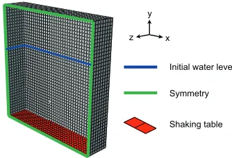
To be able to evaluate the accuracy of the different FSI methods two benchmark examples have been chosen in this project. The first, and the only one included in this paper, is a simple tank sloshing problem. The second example studied is a simplified BWR reactor, see Gasch et al. (2013). The tank sloshing example is based on the experiments presented by Goudarzi and Sabbagh-Yazdi (2012), which consisted of a series of shaking table tests of a partially water filled rectangular tank. The rectangular tank is made of 0.02 m thick reinforced acrylic glass and is 1 m high, 0.96 m long and 0.4 m wide. During the test series it was subjected to a periodic excitation in the length direction of the tank, with amplitude of 0.005 m and different frequencies and different water levels. For this benchmark example a test with a water level of 0.624 m and excitation frequency of 79.1% of the first natural frequency of the water body (approximately 4.409 rad/s) is chosen. The finite element model of the tank used in this study is shown in Figure 1. The shaking motion, 20 seconds long, is applied as a translation in the x-direction while all other DOFs at the bottom of the tank are constrained.
Symmetry Initial water level
Shaking table x
y
z
Figure 1. Finite element model of the tank including boundary conditions.
A number of different FSI methods are used in this example, ranging from purely analytical methods to advanced numerical methods. All numerical methods are available in commercial FE-software and in this study the following software have been used: ABAQUS (Dassault Systèmes, 2012), ADINA (Adina, 2011) and SOLVIA (Solvia, 2011). The methods are summarized in Table 1. Methods no. 9 and no. 10 are based on the same procedures for the structure and the fluid respectively, but for method no. 9 the equations of the fluid and the structure are solved simultaneously, while the equations in method no. 10 are solved iteratively. In both methods the fluid domain is described with an ALE-formulation and all equations are solved with an implicit time integration scheme. The elements of the fluid domain are so-called flow-condition-based-interpolation elements, which incorporate some aspects of finite volume elements into the finite element formulation, see e.g. Bathe and Zhang (2002). Due to extensive computational time, these two methods will only be analyzed in two dimensions with an almost rigid tank, hence, only the response of the fluid domain will be compared to the other analysis methods.
To increase the understanding of the behavior of the tank and the water body, frequency analyses are performed for the methods where it is possible; i.e. the linear methods. The first five natural frequencies are presented in Table 2 for analysis method no. 1, 2, 5 and 7.
Table 1: Summary of FSI methods used.
No. Method Integration Analysis type Software
1 Structure only Implicit Linear transient, Frequency Abaqus, Solvia
2 Analytical - Linear transient, Frequency -
3 Housner Implicit Linear transient Abaqus
4 Epstein Implicit Linear transient Abaqus
5 Acoustic, potential based Implicit Linear transient, Frequency Solvia, Adina
6 Acoustic, subsonic, potential based Implicit Non-linear transient Adina
7 Acoustic, velocity Implicit Linear transient, Frequency Abaqus
8 ALE, monolithic Explicit Non-linear transient Abaqus
9 ALE, monolithic Implicit Non-linear transient Adina
10 ALE, partitioned Implicit Non-linear transient Adina
Table 2: Natural frequencies from different analysis methods, first five modes.
Analysis method no. Mode number [Hz]
1st 2nd 3rd 4th 5th
1. Tank only 46.69 48.28 83.07 93.75 99.08
2. Analytical, water 0.89 - 1.56 - 2.02
5. Acoustic, water longitudinal modes 0.89 1.28 1.57 1.81 2.03
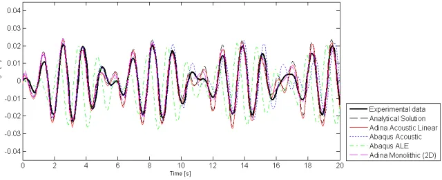
Results from the different analysis methods are compared with the experimental measurements of the free water surface as documented in Goudarzi and Sabbagh-Yazd (2012). Results from some of the analyses are presented in Figure 2. Most analysis methods show good consistency with the experimental results. Regarding all the nonlinear methods, which describe actual fluid flow, little effort has been put on adjusting numerical parameters of the analysis to obtain a more accurate solution. The purpose of this choice is to show that even though these non-linear methods have the potential to describe the flow more accurately than the acoustic, they also demand a lot more from the user to obtain good results.
Figure 2. Sloshing wave height.
The variation in the hydrodynamic fluid pressure is studied for all methods at a depth of 0.1 m below the surface close to the left wall. This should give an indication on how large load the fluid will exert on the tank wall during the periodic motion. The hydrostatic pressure at this depth is approximately 1 kPa. No measurements are available on the fluid pressure.
The maximum hydrodynamic pressure varies between 20-40 % of the hydrostatic pressure, i.e. 0.2-0.4 kPa. This magnitude is reasonable considering that the free surface varies with ±2 cm. To study how the hydrodynamic pressure varies over the height of the tank wall its vertical distribution is plotted over the height of the left tank wall in Figure 3. The pressure is shown for analysis method no. 2, 5, 7, 8 and 9 at two time points, 13.1 and 13.8 seconds, which correspond to one maximum value and one minimum value in the time histories, respectively. From both time points it can be observed that all methods give similar pressure profiles and that the largest relative increase in pressure is obtained close to the free surface. This indicates that most of the hydrodynamic pressure in this test setup comes from the convective pressure and only a small portion from the impulsive pressure, which tends to give a larger increase close to the bottom of the water body. It can also be observed that the acoustic method in Adina, method no. 5, gives the highest increase in pressure and that the acoustic method in Abaqus, method no. 7, gives the lowest increase in pressure. A significant difference between these two methods is that Adina includes the hydrostatic forces implicitly in its governing equations while Abaqus only considers the hydrodynamic pressure.
when Housner is used, which leads to larger deformations of the tank wall and thus higher stresses at that location. For the four acoustic simulations, method no. 5 to 7, the dynamic contribution of the stress state is of magnitude 2 kPa for all four simulations. The periodicity of the acoustic simulations corresponds very well with the results obtained in the simplified method according to Epstein, although the magnitude of the dynamic stress part is almost twice as large in the simplified method. In the nonlinear ALE method in Abaqus, method no. 8, a lot of high frequency noise is present throughout the entire solution. Disregarding these high frequencies it can be concluded that the dynamic part of the von Mises stress at the specified result point varies between -4 to 2 kPa, which is in good agreement with the acoustic methods.
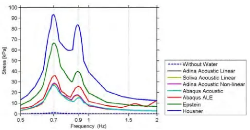
Figure 4 shows the stress response in frequency domain, i.e. response spectra. To exclude the high frequency noise in the early part of the time histories only the results from 10 to 20 seconds are considered when calculating the response spectra. The figure is zoomed in between 0.5 to 2 Hz to focus on the frequencies of the driving motion and the lower eigenmodes of the water. From the figure, two distinct peaks are visible; the first at 0.7 Hz, which coincides with the frequency of the driving motion, the second at 0.9 Hz, which corresponds to the first natural frequency of the water. Both peak values are present in the simulations which include water, but for the simulation without water only the first peak is present. It can also be observed that the magnitude is considerably higher for the simulations that include water. Further, it is shown that the two simplified methods give higher stress values at both peaks, compared with the more advanced methods. Table 3 is presented to summarize the effect of including water on the response of a structure excited by a periodic motion. The results show a significant increase in dynamic stresses in the tank wall compared to the analysis without water (method no. 1).
a) b)
Figure 3. Hydrodynamic pressure distribution against a side tank wall normalized with the hydrostatic pressure at time a) 13.1 s and b) 13.8 s.
Table 3: Increase of dynamic stress in tank wall with water included compared to method no. 1.
Method no. 3 4 5a 5b 6 7 8
Increase (×100 %) 161 100 40 40 40 40 44
CONCLUSIONS
From the comparison of the numerical methods with experimental measurements of the sloshing wave it can be concluded that all methods agree well with the experiment. Almost all methods seem to overestimate the wave height slightly, especially in the beginning of the simulation. Further, it is also evident that the beating phase where the driving frequency and the first natural frequency of the water body cancel each other is the most difficult phase to describe accurately.
Looking at the hydrodynamic pressure of the fluid, it can be concluded that it is largest close to the free surface, indicating that the hydrodynamic effects are dominated by convective pressures due to sloshing. This can be explained by the low frequency and amplitude of the driving motion, which will lead to a maximum acceleration of approximately 0.1 m/s2. By the use of the simplified methods it can be seen that the impulsive force is small compared to the resultant hydrostatic pressure in this example.
It can be concluded that it is very important to include hydrodynamic effects when considering the response of the structure when subjected to a load of periodic nature, since they will increase the load effect on the structure. Further, it can also be noted that the simplified methods, in which the hydrodynamic effects are included as a mass-spring system, resulted in much higher stresses in the structure than if the fluid was included as continuum elements. However, the more advanced methods lead to extra computational time and also require more from the analyst. With the focus of this project being the global response of the structure, most methods describe the fluid unnecessarily complicated and phenomena such as splashing against and above walls and turbulence are of little interest. The main aspects that influence the structure are the mass and inertia of the fluid along with the surface waves, the sloshing. Considering this, simplified methods such as elements with acoustic equations, and even mass-spring systems, to represent the fluid, will often suffice in giving results that are accurate enough.
REFERENCES
Adina (2011). ADINA System 8.7, ADINA R&D Inc. Watertown, MA, USA.
ASCE (1998). Seismic Analysis of Safety-Related Nuclear Structures and Commentary, ASCE Standard
4-98, American Society of Civil Engineers.
Bathe K. J., Zhang H. (2002). “A flow-condition-based interpolation finite element procedure for incompressible fluid flows”, Computer & Structures, vol. 80, pp. 1267–1277.
Belytschko T. B., Kam Liu W., Moran B. (2000). Nonlinear Finite Elements for Continua and Structures, John Wiley & Sons Ltd, England.
Benson D. J. (1992b). “Computational Methods in Lagrangian and Eulerian Hydrocodes”, Computer Methods in Applied Mechanics and Engineering, vol. 99, pp. 235-394.
Bessette G., Vaughan C., Bell R., Attaway S. (2003). “Zapotec: A Coupled Methodology for Modeling Penetration Problems”, Fluid Structure Interaction II, Wessex Institute of Technology Press, pp. 273-282.
Bøckman A., Shipilova O., Skeie G. (2012). “Incompressible SPH for free surface flows”, Computers and Fluids, vol. 67, pp. 138-151.
Dassault Systèmes (2012). Abaqus 6.12 Online Documentation, Dassault Systèmes Simulia Corp, Providence, RI, USA.
Epstein H. I. (1976). “Sesimic desing of liquid-storage tanks”, ASCE Journal of Structural Division, vol. 102, pp. 1659- 673.
Faltinsen O. M. (1978). “A numerical non-linear method of sloshing in tanks with two-dimensional flow”, Journal of Ship Research, vol. 22, pp. 193-202.
Felippa C. A., Park K. C., Farhat C. (2001). “Partitioned analysis of coupled mechanical systems”, Computer methods in applied mechanical engineering, vol. 190, pp. 3247-3270.
Gasch T., Facciolo L., Eriksson D., Rydell C., Malm R. (2013). Seismic analyses of nuclear facilities with interaction between structure and water – Comparison between methods to account for Fluid-Structure-Interaction (FSI), Report xx:xx, Elforsk AB, Stockholm, Sweden. (In press)
Gingold R.A., Monaghan J.J. (1977). “Smoothed particle hydrodynamics: theory and application to non-spherical stars”, Monthly Notices of the Royal Astronomical Society, vol. 181. pp. 375–89.
Goudarzi M. A., Sabbagh-Yazdi S. R. (2012). “Investigation of nonlinear sloshing effects in seismically excited tanks”, Soil Dynamics and Earthquake Engineering, vol. 43, pp. 355-365.
Hou G., Wang J., Layton A. (2012). “Numerical Methods for Fluid-Structure Interaction - A Review”, Communications in Computational Physics, vol. 12, no. 2, pp. 337-377.
Housner G.W. (1963). “The Dynamic Behavior of Water Tanks”, Bulletin of the Seismological Society of
America, vol. 53, no. 2, pp. 381-387.
Ibrahim R. A. (2005). Liquid sloshing dynamics: theory and applications, Cambridge University Press, USA.
Lucy L.B. (1977). “A numerical approach to the testing of the fission hypothesis”, Astronomical Journal, vol. 82, pp. 1013–1024.
Mittal R., Iaccarino G (2005). “Immersed boundary methods”, Annual Review of Fluid Mechanics, vol. 37, pp. 239-261.
Noh W. F. (1964). “CEL: A time-dependent, two-space-dimensional, coupled Eulerian-Lagrangian code”, Methods in Computational Physics, pp. 117-179, Academic Press, New York.
Olovsson L. (2000). On the Arbitrary Lagrangian-Eulerian Finite Element Method. Linköping Studies in Technology, Dissertation No. 635, Linköping University, Sweden.
Oñate E., Idelshon S.R., Celigueta M.A., Rossi R., Marti J., Carbonell J.M., Ryzhakov P., Suárez B. (2011). “Advances in the particle finite element method (PFEM) for solving coupled problems in engineering”, Computational Methods in Applied Sciences, vol. 25, pp. 1-49.
Peskin C. S. (1977). “Numerical analysis of blood flow in the heart”, Journal of computational physics, vol. 25, pp. 220-252.
Reynolds D. D. (1981). Engineering principles in acoustics: noise and vibration control, Allyn and Bacon Inc., Boston, USA.
Ross M. R. (2006). Coupling and Simulation of Acoustic Fluid-Structure Interaction Systems Using Localized Lagrange Multipliers, PhD thesis, University of Colorado.
Ryzhakov P. B., Rossi R., Idelsohn S. R., Oñate E. (2010). “A monolithic Lagrangian approach for fluid– structure interaction problems”, Computational mechanics, vol. 46, pp. 883-899.
SOLVIA (2011). SOLVIA Finite Element System Version 03, SOLVIA Engineering AB, Västerås,
Sweden.
Souli M., Benson D. J. (2010). Arbitrary Lagrangian-Eulerian and Fluid-Structure Interaction: Numerical Simulation, Wiley-ISTE, London, UK
Souli M., Zolesio M. P. (2001). “Arbitrary Lagrangian-Eulerian and free-surface methods”, Computer methods in applied mechanics and engineering, vol. 191, pp. 451-466.
Sussman T., Sundqvist J. (2003). “Fluid-Structure interaction analysis with a subsonic potential-based fluid formulation”, Computers and Structures, vol. 81, pp. 949-962.