Non-malleable Reductions and Applications
Divesh Aggarwal∗ Yevgeniy Dodis† Tomasz Kazana‡ Maciej Obremski§
January 30, 2019
Abstract
Non-malleable codes, introduced by Dziembowski, Pietrzak and Wichs [DPW10], provide a useful message integrity guarantee in situations where traditional error-correction (and even error-detection) is impossible; for example, when the attacker can completely overwrite the encoded message. Informally, a code is non-malleable if the message contained in a modified codeword is either the original message, or a completely “unrelated value”. Although such codes do not exist if the family of “tampering functions”F allowed to modify the original codeword is completely unrestricted, they are known to exist for many broad tampering familiesF. The family which received the most attention [DPW10, LL12, DKO13, ADL14, CG14a, CG14b] is the family of tampering functions in the so called (2-part)split-statemodel: here the messagex
is encoded into two sharesLandR, and the attacker is allowed toarbitrarilytamper with each
LandR individually. Despite this attention, the following problem remained open:
Build efficient, information-theoretically secure non-malleable codes in the split-state model with constant encoding rate: |L|=|R|=O(|x|).
In this work, we make progress towards obtaining this result. Specifically, we
(a) develop a generalization of non-malleable codes, callednon-malleable reductions; (b) show simple composition theorem for non-malleable reductions;
(c) build a variety of such reductions connecting various (independently interesting) tampering familiesF to each other;
(d) construct several new non-malleable codes in the split-state model by applying the com-position theorem to a series of easy to understand reductions.
In particular, we design an unconditionally secure non-malleable code with 5 parts where the size of each part is quadratic in the length of the message, and state a conjecture under which we obtain a constant rate 2 part non-malleable code in the split-state model.
Of independent interest, we show several “independence amplification” reductions, show-ing how to reduce split-state tampershow-ing of very few parts to an easier question of split-state tampering with a much larger number of parts.
Note. Some time after publishing the paper (it was presented at STOC 2015), Xin Li pointed out that one of the proofs in the paper had a mistake. In particular, we had incorrectly claimed a proof of Conjecture 26. We would like to emphasize that we still believe that Conjecture 26 is true but we do not have a proof.
∗
Department of Computer Science, National University of Singapore. Email: [email protected].
†
Computer Science Dept. NYU. Email: [email protected]. Partially supported by gifts from VMware Labs and Google, and NSF grants 1319051, 1314568, 1065288, 1017471.
‡
Institute of Informatics, University of Warsaw. Email: [email protected]. Supported by Polish National Science Centre (NCN) SONATA grant UMO-2014/13/D/ST6/03252. Partially done during postdoc visit at Computer Science Dept. NYU.
§
1
Introduction
Non-malleable codes, introduced by Dziembowski, Pietrzak and Wichs [DPW10], provide a use-ful message integrity guarantee in situations where traditional correction (and even error-detection) is impossible; for example, when the attacker can completely overwrite the encoded message. Informally, given a tampering family F, a F-non-malleable code (E, D) encodes a given message xinto a codewordy←E(x) in a way that, ify is modified intoy0=f(y) by somef ∈ F, then the messagex0 =D(y0) contained in the modified codeword y0 is either the original message x, or a completely “unrelated value”. In other words, non-malleable codes aim to handle a much larger class of tampering functions F than traditional error-correcting or error-detecting codes, at the expense of potentially allowing the attacker to replace a given message x by an unrelated messagex0 (and also necessarily allowing for a small “simulation error”ε). As shown by [DPW10], this relaxation still makes non-malleable codes quite useful in a variety of situations where (a) the tampering capabilities of the attacker might be too strong for error-detection, and, yet (b) changing xto unrelatedx0 is not useful for the attack. For example, imaginexbeing a secret key for a signa-ture scheme. In this case, tampering which keepsxthe same corresponds to the traditional chosen message attack (covered by the traditional definition of secure signatures), while tampering which changes x to an unrelated value x0 will clearly not help in forging signatures under the original (un-tampered) verification key, as the attacker can produce such signatures under x0 by himself.
Split-State Model. Although such codes do not exist if the family of “tampering functions” F
is completely unrestricted,1 they are known to exist for many broad tampering families F. One such natural family is the family of tampering functions in the so called t-split-state model St
n.
Here the k-bit message x is encoded into t shares y1, . . . , yt of length n each, and the attacker is
allowed to arbitrarily tamper with each yi individually. The rate of such an encoding is naturally
defined asτ =tn/k.
The appeal of this family comes from the fact that it seems naturally enforceable in applications, especially when t is low and the shares y1, . . . , yt are stored in different parts of memory, or by
different parties. Alternatively, non-malleable codes in this model could be interpreted as “non-malleable secret-sharing schemes”: even if all the t message shares are independently tampered with, the recovered message is either x or is unrelated to x. Not surprisingly, the setting of t= 2 appears the most useful (but also the most challenging from the technical point of view), so it received the most attention so far [DPW10, LL12, DKO13, ADL14, CG14a, CG14b, Agg15].
The known results can be summarized as follows. First, [DPW10] showed the existence of such non-malleable codes, and this existential result was further improved by [CG14a], who (amazingly!) showed that the optimal rate of such codes is just 2. Second, the work of [DPW10] also gave an efficient construction in the random oracle model. Third, the work of Liu and Lysyanskaya [LL12] built an efficientcomputationally-securenon-malleable code in the split model (necessarily restrict-ing the tamperrestrict-ing functions f1 and f2 to be efficient as well). The construction assumes so called
common reference string (CRS) which cannot be tampered, and also uses quite heavy tools from public-key cryptography, such as robust non-interactive zero-knowledge proofs [DSDCO+01] and
leakage-resilient encryption [NS09]. Thus, given the clean information-theoretic definition of non-malleable codes, we believe it is important to construct such codes unconditionally.
This was first achieved by Dziembowski, Kazana and Obremski [DKO13], who constructed an elegant non-malleable code for 1-bit messages in the split-state model. Following that, Aggarwal,
1In particular,F should not include “re-encoding functions”f(y) =E(f0
Dodis and Lovett [ADL14, Agg15] gave the first information-theoretic construction supporting k-bit messages, but where the length of each sharen=O(k7). The security proof of this scheme also
used pretty advanced results from additive combinatorics, including the so calledQuasi-polynomial Freiman-Ruzsa Theorem, which was recently established by Sanders [San12] as a step towards resolving the Polynomial Freiman-Ruzsa conjecture [Gre05]. Very recently, Chattopadhyay and Zuckerman [CZ14] construct a constant-rate non-malleable code in the 9-split-state model. How-ever, it was unclear how to reduce the number of independent parts to the optimal 2. Finally, Aggarwal, Dodis and Lovett [ADL14] stated a natural conjecture about the non-malleability of the inner product function under which one would get a 2-part split-state code with constant rate n=O(k).
Hence, prior to our work, the following question remained open (unconditionally): construct efficient, information-theoretically secure non-malleable codes in the 2-split-state model whose rate is o(k6) (and, ideally, constant).
Our Results. In this work, we make progress towards resolving this open problem, including a different conjecture (Conjecture 26) under which such constant rate codes can be constructed. In the process we developed several techniques of independent interest. Specifically, we
(a) develop a generalization of non-malleable codes, callednon-malleable reductions;
(b) show simple composition theorem for non-malleable reductions;
(c) construct a variety of such reductions connecting various (independently interesting) tamper-ing families F to each other; and
(d) construct our final, constant-rate, non-malleable code in the 2-split-state model by applying the composition theorem to a series of easy to understand reductions (one of which is currently only conjectured, but proving this appears much easier than proving the final result).
In particular, our main constructions be summarized as follows:
Theorem 1 (Main Result). (Informal) There exists efficient, information-theoretically secure non-malleable codes in the5-split-state model with quadratic size shareO(k2), wherekis the length of the message. Moreover, under Conjecture 26, there exists efficient, information-theoretically secure non-malleable codes in the2-split-state model with constant encoding rate: |L|=|R|=O(k), where k is the length of the message.
We briefly expand on these results below, but notice that our final result uses (in addition to Conjecture 26) the above mentioned recent result of Chattopadhyay and Zuckerman [CZ14] as a black-box. Without using this work, under Conjecture 26 we could directly achieve a very simple linear-rate τ = O(k) non-malleable code in the 2-split-state model, which is already considerably better than the prior state-of-the-artτ =O(k6) [ADL14, Agg15].
Non-malleable Reductions. Recall, non-malleable codes encode the message x in a way that decoding a tampered codeword either returns x itself, or yields an “independent” message x0. Abstractly, this could be viewed as “reducing” a possibly complicated family of tampering functions
F to a much simpler family NM of what we call trivial tampering functions: identity function f(x) = x and constant functions fx0(x) = x0. More generally, given two families F and G, we
perspective, non-malleable code w.r.t. to F is simply a non-malleable reduction (F ⇒ NM). More interestingly, and ignoring error terms, it is very easy to see that the notion of non-malleable reductions is transitive: (F ⇒ G) and (G ⇒ H) imply (F ⇒ H). Thus, to construct a non-malleable code w.r.t. to some possibly complicated familyF, we can define some useful intermediate families
F0=F,F1, . . . ,Fi =NM (for small constanti), and show that (F0⇒ F1), . . . ,(Fi−1 ⇒ Fi).
Aside from improved modularity, our approach has the benefit that some of our intermediate families and reductions are rather natural and could find other applications. Additionally, if a better intermediate non-malleable reduction is found in subsequent/independent work, we could immediately get an improved result for our final non-malleable code. This is precisely what hap-pened when we discovered the recent work of Chattopadhyay and Zuckerman [CZ14], which, in our terminology, gave a better non-malleable reduction from O(1)-split-state family to the trivial familyNM. Coupled with one of our constant-rate reductions from 2-split-state toO(1)-split-state family (established under Conjecture 26), the work of [CZ14] improved the rate of our final code from O(k) to O(1), giving us the desired code stated in Theorem 1 (under Conjecture 26))
Our Reductions. As we mentioned, we introduce several useful intermediate families and derive a variety of non-malleable reductions relating them. From a conceptual point of view, however, we present two incomparable non-malleable reductions (each of which is composed of several sub-reductions). Both of these reductions could be interpreted asindependence amplificationtechniques: they reduce split-state tampering of very few parts to an easier question of split-state tampering with a much larger number of parts.
Our first main result (see Theorem 18) shows a non-malleable reduction from 5-split-state tam-pering to t-split-state tampering, loosing only a factor O(t) in the rate of the code. In addition to the 5-split-state tampering, it can also tolerate so called “forgetful” family F OR5, which is
allowed to (dependently) tamper all 5 memory parts as a function of any (5−1) = 4 memory parts. (More generally, F ORt can use any (t−1) parts.) In turn, this reduction is composed of several sub-reductions, some of which are of independent interest (e.g., one reduction uses the alter-nating extraction technique of [DP07a] to reduce 2-split-state tampering to the so called family of “lookahead functions”, which is a natural model for “one-pass” tampering). We defer more detailed treatment to Section 5, here only mentioning that each of our reductions is rather elementary to state (but not prove), using only general randomness extractors or the inner product function. In particular, the resulting non-malleable codes that we get using this reduction could be “efficient” not only in theory, but even in practice.
Our second main result (see Theorem 19) is a non-malleable reduction from 2-split-state tamper-ing to the family containtamper-ingt-split-state tampering and thet-part forgetful familyF ORtmentioned above. This reduction loses a factor O(t3) in the rate, but this is still a constant when t= O(1). Also, although the proof of this reduction is, by far, the most technically involved part of this work, the reduction itself is very simple and efficient, using only the inner product function. Un-fortunately, as of present one of our intermediate reductions is only conjectured to be secure (see Conjecture 26), so the final result is still conditional. We hope future work will prove Conjecture 26, and make our final result unconditional. We defer more detailed discussion to Section 6.
model.
Second, we can now compose this code with our second reduction (from 2 parts to t= 5 parts or the forgetful familyF OR5) to get still quite simple linear rate non-malleable code in the 2-split-state model (under Conjecture 26). As we mentioned, this already considerably improves the prior state-of-the-artO(k6) rate code by [ADL14, Agg15].
Finally, instead of our own non-malleable code in thet= 5 split-state model above, we can use the beautiful recent work of [CZ14], which uses a variety of advanced techniques to construct a constant-rate non-malleable code in the 9-split-state model (i.e., number of partst= 9). Composing this constant-rate code with our second reduction from 2 tot= 9 part, which only loses a constant factor in the rate, we get our final code claimed in Theorem 1 (and, formally, in Theorem 23, established under Conjecture 26).
Other Related Work. Other results that look at an (enhanced) split-state model are Faust et al. [FMNV14] which consider the model where the adversary can tamper continuously, and [ADKO15], that considers the model where the adversary, in addition to performing split-state tampering, is also allowed some limited interaction between the two states.
In fact, the result of [ADKO15] combined with our result gives a constant rate non-malleable code that also allows leakage of a 1/12-th fraction of the bits from one share of the codeword to the other. In addition to the already-mentioned results, several recent works [CCFP11, CCP12, CKM11, FMVW14, AGM+14, AGM+15] either used or built non-malleable codes for various fam-ilies F, but did not concentrate on the split-state model, which is our focus here.
The notion of non-malleability was introduced by Dolev, Dwork and Naor [DDN00], and has found many applications in cryptography. Traditionally, non-malleability is defined in the com-putational setting, but recently non-malleability has been successfully defined and applied in the information-theoretic setting (generally resulting in somewhat simpler and cleaner definitions than their computational counter-parts). For example, in addition to non-malleable codes studied in this work, the work of Dodis and Wichs [DW09] defined the notion of non-malleable extractors as a tool for building round-efficient privacy amplification protocols.
Finally, the study of non-malleable codes falls into a much larger cryptographic framework of providing counter-measures against various classes of tampering attacks. This work was pioneered by the early works of [ISW03, GLM+03, IPSW06], and has since led to many subsequent models. We do not list all such tampering models, but we refer to [KKS11, LL12] for an excellent discussion of various such models.
Subsequent Work. Following our work, there have been results that have obtained near optimal non-malleable codes in the split-state model. In particular, there have been non-malleable codes in the 2-split-state model with near constant rate [AB16, CGL16, Li17] and non-malleable codes in the 3-split state model with rate being a small constant [KOS17, KOS18, GMW18].
Additionally, there have been some results that have obtained non-malleable codes against continuous tampering in the split-state model [AKO17, ADN+17].
2
Preliminaries
For a setT, letUT denote a uniform distribution overT, and, for an integer`, letU`denote uniform
distribution over`bit strings. Thestatistical distancebetween two random variablesA, Bis defined by ∆(A; B) = 12P
v|Pr[A=v]−Pr[B=v]|. We use A≈εB as shorthand for ∆(A, B)≤ε.
The min-entropy of a random variable W is H∞(W)
def
= −log(maxwPr[W = w]), and the
conditional min-entropy ofW given Z isH∞(W|Z)
def
=−log (Ez←ZmaxwPr[W =w|Z =z]).
Definition 3. We say that an efficient function Ext : {0,1}N × {0,1}d → {0,1}n is an
(N, m, d, n, ε)-extractor if for all sources (W, Z) of conditional min-entropy H∞(W|Z) ≥ m, we
have (S, Z,Ext(W;S))≈ε(S, Z, Un), where S is uniform on {0,1}d.
In Section 5, we will be concerned with the case when d=n(seed length equals output length), and will use the existence of the following extractors:
Lemma 4 ([GUV07]). There exist constants c1 and c2, such that for any N and n satisfying
n ∈ [c1 ·logN, N/2], there exists an explicit, efficient (N, m = 2n, d =n, n, ε = 2−c2·n)-extractor
Ext.
We also also use bit-extractors which extract only one bit. One such extractor is the bit inner product function hW, Si (which trivially follows from the Leftover Hash Lemma [HILL99]). We state this below, for future convenience renaming the source length ton(and no longer using nfor output size, as the latter is 1):
Lemma 5. The inner product function is an(n, m, n, `,2−(m−`−1)/2)-extractor.
Definition 6. We say that a functionExt : {0,1}n× {0,1}n→ {0,1}m is an(n, k, m, ε)-2-source
extractorif for all independent sourcesX, Y ∈ {0,1}nsuch that min-entropyH
∞(X)+H∞(Y)≥k,
we have (Y,Ext(X, Y))≈ε(Y, Um), and(X,Ext(X, Y))≈ε(X, Um).
For n being an integer multiple of m, and interpreting elements of {0,1}m as elements from F2m and those in {0,1}n to be from (F2m)n/m, we have that the inner product function is a good
2-source extractor.
Lemma 7. For all positive integers m, n such that n is a multiple of m, and for all ε >0, there exists an efficient (n, n+m+ 2 log 1ε, m, ε) 2-source extractor.
We will need the following results. We include proofs in Appendix A for completeness. The following is a simple result from [ADL14].
Lemma 8. LetX1, Y1 ∈ A1, andY1, Y2 ∈ A2 be random variables such that∆((X1, X2) ; (Y1, Y2))≤
ε. Then, for any non-empty setA0 ⊆ A1, we have
∆(X2|X1 ∈ A0 ; Y2 |Y1 ∈ A0)≤
2ε Pr(X1 ∈ A0)
.
The following result is from [DP07a].
Lemma 9. Let A∈ AandB ∈ B be two independent random variables. Let V1, V2, . . . be random
variables defined as functions of A, B satisfying the following property. For all i∈ N, if i is even then Vi = φi(V1, . . . , Vi−1, A) and if i is odd, then Vi = φi(V1, . . . , Vi−1, B) for some function φi.
Then for all i, A is independent ofB given V1, . . . , Vi.
The following is (a generalization of) the Vazirani’s XOR Lemma.
Lemma 10. Let X = (X1, . . . , Xt) ∈ Ft be a random variable, where F is a finite field of order
q. Assume that for all a1, . . . , at ∈ Ft not all zero, ∆(Pit=1aiXi ; U) ≤ ε, where U is uniform
in F. Then ∆(X1, . . . , Xt ; U1, . . . , Ut) ≤εq(t+2)/2, where U1, . . . , Ut are independent and each is
3
Non-malleable Reductions and Useful Tampering Families
Definitions. In the following we generalize the notion of non-malleable codes w.r.t. to a
tam-pering family F [DPW10] to a more versatile notion of non-malleable reductionsfrom F toG.
Definition 11 (non-malleable reduction). Let F ⊂ AA and G ⊂ BB be some classes of functions (which we call manipulation functions). We will write:
(F ⇒ G, ε)
and say F reduces to G, if there exist an efficient randomized encoding functionE :B → A, and an efficient deterministic decoding function D : A → B, such that (a) for all x ∈ B, we have D(E(x)) =x, and (b) for all f ∈ F, there existsGsuch that for all x∈B,
∆D(f(E(x))) ; G(x)≤ε, (1)
whereG is adistributionoverG, and G(x) denotes the distributiong(x), whereg←G. The pair (E, D) is called (F,G, ε)-non-malleable reduction.
Intuitively, (F,G, ε)-non-malleable reduction allows one to encode a value x by y ← E(x), so that tampering withybyy0 =f(y) forf ∈ F gets “reduced” (by the decoding functionD(y0) =x0) to tampering withx itself via some (distribution over) g∈ G.
In particular, the notion of non-malleable code w.r.t. F, is simply a reduction from F to the family of “trivial manipulation functions”NMk defined below.
Definition 12. LetNMk denote the set of trivial manipulation functions on k-bit strings, which
consists of the identity function I(x) =x and all constant functionsfc(x) =c, wherec∈ {0,1}k.
We say that a pair (E, D) defines an (F, k, ε)-non-malleable code, if it defines a (F,NMk,
ε)-non-malleable reduction.
Remark 1. The above definition might seem a little different than the definition of [DPW10] (who required a simulator outputting a distribution over constantsc∈ {0,1}k, a special symbol “same”,
serving as a disguise for the identity function, and another special symbol ⊥). The symbol ⊥ is meant to indicate that the tampered codeword is invalid, and facilitates one to view non-malleable codes as a relaxation of error-detecting codes, where one wants to detect tampering. However, one can equivalently consider the non-malleable code defintion without⊥, simply by replacing the “bottom output”⊥by a fixed message whenever the simulator or decoder outputs⊥. We formally discuss this issue in Appendix B, where we also show the equivalence between the definition of non-malleable code presented here and the one in [DPW10].
Remark 2. Notice, the “complexity” of the initial tampering familyF intuitively corresponds to the complexity of the attacker on our system. Hence, when F consists of efficient functions (and so does the target family G; e.g. G =NMk), it could be useful to require that the distribution G
overG is efficiently samplable given oracle access to f ∈ F. However, we do not insist on this for two reasons: (1) our final tampering family F (the split-state family) will consist of arbitrary and possibly inefficient functions f, making the efficiency requirement onG less motivated; and, more importantly, (2) for the reduction from any family F to the trivial familyNMk (which is our final
Lemma 13. Let (E, D) be an (F, k, ε)-non-malleable code for some tampering family F. Then for allf ∈ F, there exists a random function G distributed over NMk such that for all x∈ {0,1}k,
∆D(f(E(x))) ; G(x)≤2ε+ 1 2k ,
and G is efficiently samplable given oracle access to f.
We also give a related useful notion of non-malleable transformations, where theF-tampering is applied touniformly randomstrings inA, and gets transformed (by some “transformation function” T) to G-tampering over uniformly randomstrings inB.
Definition 14 (non-malleable transformation). LetF ⊂AAand G ⊂BB be some classes of manipulation functions. We will write:
(F → G, ε)
and sayF transforms to G, if there exists an efficienttransformation functionT :A→B such that for all f ∈ F there existsG such that:
∆
T(f(UA)), T(UA) ; G(UB), UB
≤ε, (2)
whereG is a distribution overG, and G(x) denotes the distribution g(x), whereg←G. The function T is called (F,G, ε)-non-malleable transformation.
Remark 3. Equation (2) implies the following analog of “correctness”: ∆T(UA);UB
≤ε.
The utility of non-malleable reductions and transformations comes from the following natural composition theorem, which allows to gradually make our tampering families simpler and simpler, until we eventually end up with a non-malleable code (corresponding to the trivial familyNMk).
Theorem 15 (Composition). (a) If (F → G, ε1) and (G → H, ε2), then (F → H, ε1+ε2).
(b) Similarly, if (F ⇒ G, ε1) and (G ⇒ H, ε2), then (F ⇒ H, ε1+ε2).
Proof. We give the proof for (slightly more involved) part (b), as the proof for part (a) is analogous. Since (F ⇒ G, ε1), there exists functions (E1, D1) satisfying Equation (1), and same for (E2, D2)
for (G ⇒ H, ε2). We claim that (E1◦E2, D2◦D1) is a correct reduction for (F ⇒ H, ε1+ε2). The
correctness property is obvious, and the security follows from these equations:
((D2◦D1)(f((E1◦E2)(x)))) = (D2(D1(f(E1(E2(x))))))≈ε1 D2(G(E2(x)))≈ε2 H(x)
which means
((D2◦D1)(f((E1◦E2)(x))))≈ε1+ε2 H(x),
as needed.
We will also need the following trivial observation.
Observation 1 (Union). Let (E, D) be an (F,H, ε) and a (G,H, ε0) non-malleable reduction (resp. transformation). Then (E, D) is an (F ∪ G,H,max(ε, ε0)) non-malleable reduction (resp. transformation).
Theorem 16. Let F ⊂AA,G ⊂BB. Assume (F → G, ε) with transformation T. For anyx∈B, let T−1(x) denote a uniformly random element U in A such that T(U) = x. If for all x ∈ B,
T−1(x) is efficiently samplable, then (F ⇒ G,2ε|B|).
Proof. We define D:A7→B to beT andE is defined asE(x) :=T−1(x) for allx∈B. Then the correctness is obvious. Consider somex∈B. Using Equation 2 and Lemma 8, we have that
∆(D(f(UA))|D(UA) =x; G(UB)|UB=x)≤
2ε Pr(UB =x)
,
which implies
∆(D(f(E(x))) ; G(x))≤2ε|B|.
Useful Tampering Families. We define several natural tampering families we will use in this
work. For this, we first introduce the following “direct product” operator on tampering families:
Definition 17. Given tampering families F ⊂ AA and G ⊂ BB, let F × G denote the class of functions hfrom (A×B)A×B such that
h(x) =h1(x1)||h2(x2)
for someh1 ∈ F and h2∈ G and x=x1||x2, wherex1∈A, x2∈B.
We also let F1 :=F, and, for t≥1, Ft+1:=Ft× F.
We can now define the following tampering families:
• Sn= ({0,1}n){0,1} n
denote the class of allmanipulation functions onn-bit strings.
• Given t > 1,St
n denotes the tampering family in the t-split-state model, where the attacker
can apply t arbitrarily correlated functions h1, . . . , ht to t separate, n-bit parts of memory
(but, of course, eachhi can only be applied to the i-th part individually).
• F ORtn denotes forgetful family. It is applied to t parts of memory of length n but the output value can depend only on (t−1) parts. More precisely: Let x ∈ {0,1}tn be a bit
vector and xi ∈ {0,1}n denote i-th block of n bits. For anyh ∈ F ORtn there exist a subset
S ⊂ {1,2, . . . , t} of size (t−1) such thath(x) can be evaluated from xS. Besides that, it is
not restricted in any way.
• Finally,LA←tn ⊂({0,1}tn){0,1}tn
denotes the class oflookahead manipulation functionslthat can be rewritten asl= (l1, . . . , lt), for li:{0,1}in → {0,1}n, where
l(x) =l1(x1)||l2(x1, x2)||. . .||li(x1, . . . , xi)||. . .||lt(x1, . . . , xt)
for x = x1||x2||. . .||xt, and xi ∈ {0,1}n. In other words, if l(x1, . . . , xt) = y1, . . . , yt, then
each yi can only depend on the “prior”x1, . . . , xi.
4
Our Reductions and Application to Non-malleable Codes
Our Reductions. In this Section, we state our main reductions. Both our reductions could be interpreted asindependence amplificationtechniques: they reduce split-state tampering of very few parts to an easier question of split-state tampering with a much larger number of parts. Our first result shows a non-malleable reduction from 5-split-state tampering tot-split-state tampering.
Theorem 18 (Independence amplification from 5 parts). (S5
12t2 ⇒ S1t,2−Ω(t)).
In our second result, we show a non-malleable reduction from 2-split-state tampering to the family containing t-split-state tampering and thet-part forgetful family. This result is not uncon-ditional, but relies on a Conjecture 26 we explain later.
Theorem 19 (Independence amplification from 2parts). Assuming Conjecture 26, we have that(S2
O(t4n)⇒ Snt ∪ F ORtn,2−Ω(n)).
Theorem 18 will be proved in Section 5 and Theorem 19 will be proved in Section 6.
Application to Non-malleable Codes. We can compose the reduction in Theorem 18 with the already known constructions of non-malleable codes in the independent-bit tampering model (i.e. for tampering families Sk
1), summarized below [DPW10, CG14b, FMVW14, AGM+15]:
Theorem 20 (NM code for bit tampering [CG14b]). (S1.1k
1 ⇒NMk,2−Ω(k)).
Using Theorem 15, and Theorem 18 with t=k, we get the following result:
Theorem 21 (5-split NM code with rate O(k)). There exists an efficient(S5
O(k2), k,2
−Ω(k)
)-non-malleable code, i.e.,
(SO5(k2)⇒NMk,2−Ω(k)).
Using a recent work of Chattopadhyay and Zuckerman [CZ14]. [CZ14] obtained a construction of non-malleable codes with constant rate in the 9-split-state model. Their construction was achieved using a connection of t-source non-malleable extractors to non-malleable codes in the t-split-state model shown in [CG14b]. We observe that if the extractor is also a strong extractor (which is the case for [CZ14]), then the corresponding code is also non-malleable against the forgetful family. The details can be found in Appendix C, but they imply the following result:
Theorem 22 (9-split NM code with rate O(1)). There exist n = O(k), such that (S9 n∪
F OR9
n⇒NMk,2−Ω(k)).
Combining this with our reduction given in Theorem 19, we get our main result.
Theorem 23 (Main result: 2-split NM code with rate O(1)). Assuming Conjecture 26, we have that (S2
O(k) ⇒ NMk,2
−Ω(k)), i.e, there exists and efficient (S2
O(k), k,2
−Ω(k))-non-malleable
code.
5
Non-Malleable Reduction from 5 parts to t parts
5.1 Our Construction
composition theorem (Theorem 15). We now specify the intermediate steps, leaving the proofs of corresponding theorems to subsequent subsections.
Our first result is a transformation from 2-split-state model to the “t-lootahead model”. Namely, we gain in introducing many parts, at the expense of dealing with more challenging tampering functions on each part (as compared to the split-state model).
Theorem 24 (2-split to lookahead). (S2
3tn→ LA←tn , t2·2−Ω(n)).
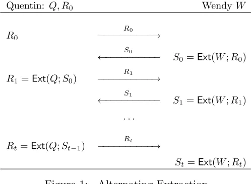
The proof is given in Section 5.2, but here we briefly sketch the definition of the required transformation T1 (see Section 5.2 for more details). It is based on the alternating extraction
protocol [DP07b] depicted in Figure 1. The first memory part stores random strings Q, R0, the
second memory part stores randomW (where |Q|=|W| ≈2tnand |R0|=n), and we let
T1((Q, R0), W) = (R1, . . . , Rt), (3)
where eachRiis iteratively defined by usingRi−1to extractSi−1fromW, and thenSi−1to extract
Ri from Q.
Next, we show how to transform two independentt-lookahead tampering families to the t-split-state tampering family (and, for future use, the forgetful family).
Theorem 25 (2-lookahead to t-split). If n≥4t, then
(LA←tn × LA←tn → S1t, O(2−Ω(n))).
The proof is given in Section 5.3, but here we only mention the definition of the transformation T2 we construct. Let Ext2 be any (n, n/2 + 1, n,1,2−n/4)-extractor (e.g., the inner product), and
define
T2(L, R) := (Ext2(Lt, R1),Ext2(Lt−1, R2), . . . ,Ext2(L1, Rt)), (4)
whereL= (L1||. . .||Lt), R= (R1||. . .||Rt), Li, Ri∈ {0,1}n.
Intuitively, it seems that the result of Theorem 25 reveals that it should be possible to extend the result to a reduction from 2 lookahead to t split, where t is a constant and each split state is O(n). However, the current proof technique is not able to achieve this. We conjecture the following:
Conjecture 26 (2-lookahead to t-split). There exist a universal constant C such that the following holds. If n≥Cmt, then
(((LA←tn × LA←tn )∪ F OR2nt)→(Smt ∪ F ORtm), O(2−Ω(n))).
We remark that it is trivial to see that the reduction of this Section also gives
(F OR2nt→ F ORtm,2−(n−m−1)/2).
This is because by the strong extractor property of Ext2, for anyi, Ext2(Li, Ri) is 2−Ω(n) close to
uniform given
L1, . . . , Li−1, Li+1, . . . , Lt, R1, . . . , Ri−1, Ri+1, . . . , Rt,
and one ofLi, Ri.
As a direct corollary of Theorems 24 and 25, we get a transformation from 4-split-state model tot-split state model:
Theorem 27. (S4
Now, it is tempting to use Theorem 16 to get a non-malleable reduction from S4
12t2 to S1t.
Unfortunately, we do not know how to turn the non-malleabletransformationin Theorem 27 into a reduction(i.e., how to efficiently invertT in Theorem 27, and then apply Theorem 16). Instead, we observe the following very general result allowing us to translate a non-malleable transformation from any F to t-split tampering St
1, into a non-malleable reduction from F × St to S1t. Namely,
in thet-split model, we go from transformation to reduction at the expense of another “split-state part” St.
Theorem 28. If (F → St
1, ε), then (F × St⇒ S1t,2ε).
In particular, using the transformation in Theorem 27, we get
(S5
12t2 ⇒ S1t,2−Ω(t)).
The proof is given in Section 5.4, but we briefly mention the reduction (E, D) as a function of the transformation T. To encode a valuex∈ {0,1}t, we pick a randomy in the domain ofF, and
let x∗ =T(y), d=x⊕x∗, and output (y, d) (where dis stored in the extra t-bit part). To decode (y, d), we compute D(y, d) =T(y)⊕d.
Of course, by using “dummy” bits to extend the 5-th part from t bits to 12t2 bits, we get a reduction from 5-split-state model tot-split state model.
5.2 From two split-state parts to lookahead (proof of Theorem 24)
We first recall the alternating extraction, which was introduced by Dziembowski and Pietrzak in [DP07b], and present a particular variant of the alternating-extraction theorem from Dodis and Wichs [DW09], which will be especially convenient for our purposes. We then show how to use this result to get our non-malleable transformation.
Quentin: Q, R0 WendyW
R0
R0
−−−−−−−−−−→
S0
←−−−−−−−−−− S0=Ext(W;R0) R1=Ext(Q;S0)
R1
−−−−−−−−−−→
S1
←−−−−−−−−−− S1=Ext(W;R1) . . .
Rt=Ext(Q;St−1)
Rt
−−−−−−−−−−→
St=Ext(W;Rt) Figure 1: Alternating Extraction
Alternating Extraction. Assume that two parties, Quentin and Wendy, have uniformly random N-bit valuesQand W, respectively, such thatW is kept secret from Quentin andQ is kept secret from Wendy. Let Ext be the efficient (N,2n, n, n,2−Ω(n))-extractor given in Lemma 4 (where n= Ω(logN)), and assume that Quentin also has a random seedR0 ∈ {0,1}nfor the extractorExt.
R1 = Ext(Q;S0). In each subsequent iteration i, Quentin sends Ri to Wendy, who replies with
Si = Ext(W;Ri), and Quentin computes Ri+1 = Ext(Q;Si). Thus, Quentin and Wendy together
produce the sequence:
R0, S0 =Ext(W;R0), R1 =Ext(Q;S0), . . . , Rt=Ext(Q;St−1), St=Ext(W;Rt) (5)
The alternating-extraction theorem says that there is no better strategy that Quentin and Wendy can use to compute the above sequence. More precisely, for our purposes we will use the following version (slightly weaker than the most general version presented by [DW09]). Let us assume that, in each iteration, Quentin is limited to sending at most s bits to Wendy, who can then reply by sending at mostsbits to Quentin, wheresis much smaller than the entropy (i.e., length)N ofQand W (preventing Quentin from sending his entire value Q, and vice versa). Then, for any possible strategy cooperatively employed by Quentin and Wendy in the first i iterations, the value Si+1
(and alsoSi+2, . . . , St, but we won’t use it) look uniformly random to Quentin (and, symmetrically,
Ri+1, and even Ri+2, . . . , Rt look random to Wendy). In other words, Quentin and Wendy acting
together cannot speed up the process in some clever way, so that Quentin would learn Si+1 (or
even distinguish it from random) in fewer than i+ 1 iterations.
More formally, the following variant of alternating extraction Theorem is a special case of Lemma 41 from [DW09].
Theorem 29 (Alternating Extraction; [DP07b, DW09]). For any integers N, n, s, t, where N ≥st+ 2n and n = Ω(logN), let W, Q be two random and independent N-bit strings, and Ext
be an efficient (N,2n, n, n, ε= 2−Ω(n))-extractor (which exists by Lemma 4). Let R0 be uniformly
random on {0,1}n and define S
0, R1, S1, . . . , Rt, St as in equation (5). Let Aq(Q, R0),Aw(W) be
interactive machines such that, in each iteration, Aq sends at most sbits to Aw which replies with
at most s bits to Aq. Let Vwi, Vqi denote the views of the machines Aw,Aq respectively, including their inputs and transcripts of communication, after the first i iterations. Then, for all 0≤i≤t,
Vwi, Ri
≈2tε Vwi, Un
and Vqi, Si
≈2tε Vqi, Un
(6)
Our Non-Malleable Transformation. In the proof, we will use the alternating extraction theorem with per round communication s= 2n, so that we can set N = 2nt+ 2n. Our first part of memory will simply random Q ∈ {0,1}N and R
0 ∈ {0,1}n, and the second part will store a
random W ∈ {0,1}N, so that the size of each memory piece is at most N +n ≤ 3tn (which is
what is claimed in Theorem 24), and our non-malleable transformationT1((Q, R0), W) will simply
output tstrings (R1, . . . , Rt), as defined in the alternating extraction protocol.
Now, let us fix arbitrary tampering functionsfq(Q, R0) = (Q0, R00) andfw(W) =W0 on the two
memory parts, and let (R01, . . . , R0t) denote the output of an (honest) execution of the alternating extraction protocol on inputs (Q0, R00) and W0. To complete the proof, it suffices to show the validity of Equation (2). Namely, for given fq and fw, we need to exhibit a distribution G over
“lookahead functions”g(P1, . . . , Pt) =g1(P1)||g2(P1, P2)||. . .||gt(P1, . . . , Pt) such that
∆
(R1, R01, . . . , Rt, R0t) ; (P1, P10, . . . , Pt, Pt0)
≤t2·2−Ω(n), (7)
where eachPi≡Un (uniformn-bit string) and (P10, . . . , Pt0) =G(P1, . . . , Pt).
We describe the distribution G as a stateful probabilistic algorithm which, given P1, produces
P10, then additionally given P2, produces P20, etc., which is equivalent to the lookahead restriction
si−1, Pi = si, it samples (using fresh independent coins) the value s0i from the “real” conditional
distribution
Ri0 |(R1 =s1, R01 =s 0
1, . . . , Ri−1 =si−1, R0i−1=s 0
i−1, Ri =si),
and outputs Pi0 = s0i. Namely, G views its inputs sj, which are actually sampled uniformly at
random fromUn, as if coming from the “correct distribution” of running the alternating extraction
protocol on random Q, R0, W. And then G samples the tampered value s0i under this (incorrect)
assumption.
To argue Equation (7), we use the hybrid argument and definet+ 1 intermediate distributions D0, . . . , Dt, where D0 = (R1, R01, . . . , Rt, R0t), Dt = (P1, P10, . . . , Pt, Pt0), while the intermediate
distributionDi is defined as follows. For the firstisteps, it honestly samples values (Ri, R0i) from
the left distribution, while for the last (t−i) steps it takes the partial history (s1, s01, . . . , sj−1, s0j−1)
so far, picksuniformly randomsj ←Un, and sampless0j from the conditional distribution described
above (using fresh coins every time). We can indeed see that D0 = (R1, R01, . . . , Rt, R0t), Dt =
(P1, P10, . . . , Pt, Pt0), so it suffices to show that ∆(Di;Di+1)≤2tε, where ε= 2−Ω(n) is the same as
in Theorem 29.
Fortunately, this immediately follows from the alternating extraction theorem above, using the following machines Aq(Q, R0),Aw(W). Aq(Q, R0) computes (Q0, R00) = fq(Q, R0), and runs
two honest executions of the alternating extraction protocol with real input (Q, R0) and tampered
input (Q0, R00), andAw(W) does the same thing on its side. This indeed gives communication bound
s= 2nper round, and also results in a viewVwi which includes precisely (R1, R01, . . . , Ri, Ri0). Hence,
using Equation (6), we get
R1, R01, . . . , Ri, R0i, Ri+1
≈2tε R1, R01, . . . , Ri, Ri0, Un
,
which is precisely the (i+1)-prefixes of our distributionsDiandDi+1. But since the (t−i−1)-suffixes
are sampled in the same way for both distributions, applying Lemma 2 yields ∆(Di;Di+1) ≤2tε,
completing the proof of Theorem 24.
5.3 From two look-ahead parts to t-split (proof of Theorem 25)
In this section, we show that if n≥4t, then (LA←tn × LA←tn ∪ F OR2t
n → S1t∪ F ORt1, t·2− n 4).
Notation for the proof. Let Li, Ri ∈ {0,1}n be random vectors, and let Ext2(Li, Ri) = bi ∈
{0,1}. Define:
L:= (Lt, Lt−1, . . . L1) R:= (R1, R2, . . . Rt)
Consider the output after applying manipulation function from LA←tn × LA←tn to L and R. (Notice, we will generally use primed letters for manipulated values.) It can be described as:
L0i:=fi(Li, Li+1, . . . , Lt) R0i :=gi(R1, R2, . . . , Ri)
for some set of functions (called manipulation family) f1, g1, f2, g2, . . . ft, gt. Notice, whileR0i
de-pends on R1, . . . , Ri, the value Li0 depends on Li, . . . , Lt, since we “reversed” the vector L above,
so that the manipulation function from LA←tn reads the values of L“backwards”. Similar notation will be used for decoding of manipulated input bitstrings:
We need to prove that
(b1, b01, . . . , bt, b0t)≈t2−n/4 (U(1), h1(U(1), Z1). . . , U(t), ht(U(t), Zt)), (8)
where U(1), . . . , U(t) denote independent random elements in {0,1}, andZ = (Z1, . . . , Zt) is some
random variable independent ofU(1), . . . , U(t). Note thatZ1, . . . , Ztmight have dependence amongst
themselves. In order to prove this, we need to define Z1, . . . , Zt, which we do below.
Definition of Z. We define random variables Z1, . . . , Zt iteratively.
Define Var1 to be the joint random variable (L2, . . . , Lt). Let Y1 be a fresh random variable
that samples the distributionL1 given the values ofVar1,R1 andExt2(L1, R1). Thus, conditioned
on R1,Ext2(L1, R1),Var1, we have
L1 ≡φ1(Var1, R1, Y1,Ext2(L1, R1)),
for some functionφ1. DefineZ1= (Z1,b :b∈ {0,1}) indexed by bto be a 2-bit random variable as
a function ofR1,Var1, Y1 as follows:
Z1,b:=Ext2(f1(φ1(Var1, R1, Y1, b), L2, . . . , Lt), g1(R1)) .
Note thatb01 =Z1,b1 is a deterministic function ofZ1 and b1. Letb
0
1=h1(b1, Z1).
Now, given Z1, . . . , Zi−1, we defineYi, Zi. DefineVari to be the joint random variable
Vari =Z1, . . . , Zi−1, R1, . . . , Ri−1, Li+1, . . . , Lt.
LetYi be a fresh random variable that samples the distributionLi given the values ofVari,Ri, and
Ext2(Li, Ri). Thus, conditioned onRi,Ext2(Li, Ri),Vari, we have
Li≡φi(Vari, Ri, Yi,Ext2(Li, Ri)),
for some function φi. DefineZi = (Zi,b :b∈ {0,1}) indexed by b to be a 2-bit random variable as
a function ofRi,Vari, Yi as follows:
Zi,b:=Ext2(fi(φi(Vari, Ri, Yi, b), Li+1, . . . , Lt), gi(R1, . . . , Ri)) .
Note thatb0i =Zi,bi is a deterministic function ofZi and bi. Letb 0
i =hi(bi, Zi).
Proof of Theorem. We prove Equation (8) using a hybrid argument. In particular, we show that for alli= 1, . . . , t,
(U(1), h1(U(1), Z1), . . . , U(i−1), hi−1(U(i−1), Zi−1), bi, b0i, bi+1, b0i+1, . . . , bt, b0t)
≈2−n/4(U(1), h1(U(1), Z1), . . . , U(i−1), hi−1(U(i−1), Zi−1), U(i), hi(U(i), Zi), bi+1, b0i+1, . . . , bt, b0t).
(9)
Equation (8) then follows from (9) by triangle inequality.
To prove Equation (9), consider the following. Since the total length ofZ1, . . . , Zi−1is 2(i−1)≤
2(t−1)≤ n2 −2, we have thatH∞(Li|Vari) =H∞(Li|Z1, . . . , Zi−1)≥ n2 + 2. Also notice that Ri
is independent of Vari. Indeed, tracing the definition of Z1, . . . , Zi−1 and using the “lookahead”
property ofR, we see that functions g1, . . . , gi−1 were only applied to R1, . . . , Ri−1 when defining
and also throwing completely fresh and independent values U(1), . . . , U(i−1), Yi, Ri+1, . . . , Rt into
the mix, we can apply Lemma 5 and get
(Z1, . . . , Zi−1, U(1), . . . , U(i−1), Ext2(Li, Ri),R1, . . . , Ri, Yi, Ri+1, . . . , Rt, Li+1, . . . , Lt)
≈2−n/4(Z1, . . . , Zi−1, U(1), . . . , U(i−1), U(i), R1, . . . , Ri, Yi, Ri+1, . . . , Rt, Li+1, . . . , Lt) .
(10)
We now claim that Equation (9) directly follows from Equation (10) by applying Lemma 2. To see this, we notice that, by the “lookahead”property of L, the values bi+1, b0i+1, . . . , bt, b0t are
deterministic functions ofR1, . . . , Rt, Li+1, . . . , Lt (in particular, they do not depend onLi). Also,
the value Zi is deterministic function of Yi, Z1, . . . , Zi−1, R1, . . . , Ri, Li+1, . . . , Lt (in particular, it
also does not depend on the Li). Finally, bi =Ext2(Li, Ri) andb0i =hi(bi, Zi), which means that
(bi, b0i) (resp. (U(i), hi(U(i), Zi))) is also a deterministic function ofExt2(Li, Ri), Zi (resp. U(i), Zi).
This concludes the proof of the fact that (LA←tn × LA←tn → St
1, t·2−n/4), as all variables in the
left (resp. right) hand side of Equation (9) are deterministic functions of the same corresponding variables from left (resp. right) hand side of Equation (10).
5.4 From transformation to reduction fort-split state tampering (proof of The-orem 28)
LetF ⊂AAand T be a function given by definition of non-malleable transformation (F → St 1, ε).
We start with definitions of encoding and decoding functions that we claim satisfy the definition of a non-malleable reduction. Let E :{0,1}t → A× {0,1}t : be a random experiment defined as
follows:
E(x) :=ny←−$ A ; x∗ :=T(y) ; d:=x⊕x∗ ; Output (y, d)o
and corresponding decoding:
D(y, d) :=T(y)⊕d.
It is obvious that both encoding and decoding are efficient and thatD(E(x)) =xfor allx∈ {0,1}t.
Proof of reduction property. We need also to prove Equation (1). Let us fixx, and tampering functions f ∈ F and g∈ St. We denote the tampered values with primed letters. SinceT(y) =x∗
and F transforms to St
1, Equation (2) implies that with probability at least (1−ε) all the values
(x∗i)0 = fi(x∗i) (for some functions (f1, . . . , ft) distributed over S1t). Also let d0 := g(d) be the
tampered value of the last part. Then, ignoring the ε-failure event above (for which we will payε in the statistical distance), we have:
x0i=d0i⊕(x∗i)0 =g(d)i⊕fi(x∗i) =g(d)i⊕fi(xi⊕di) =hi(xi, d)
for some function hi. To complete the argument, it remains to argue that d is “ε-independent”
fromx(i.e., (x, d)≈ε(x, Ut)), meaning thathiisε-close to a valid independent tampering function.
However, this follows again from Equation (2), sinced=x⊕x∗, andx∗ isε-close toUt (even given
x, sincey ←Ais random and independent from x).
Thus,x0 is indeed 2ε-close to a convex combination of functions fromSt
1 applied tox.
6
Non-Malleable Reduction from 2 parts to t parts
Theorem 30. (S2
10t(t2+t+1)(n+3ts)⇒(LA
←t/2
n × LA←t/n 2)∪ F ORtn, O(t4·2−s)).
This result (whose proof will take the remainder of this section, and which is by far the most complicated individual reduction that we construct) can be seen as strengthening of Theorem 24. Namely, while Theorem 24 reduced 2-split-state tampering to a single lookahead tampering, in our new reduction we manage to reduce it to two independentlookahead tamperings.2
To prove Theorem 30, we need to define encoding and decoding functions (see Definition 11) and prove that they satisfy the required conditions for non-malleable reductions. Correspondingly, in Section 6.1 we will first define our efficient reduction, and then prove its security in Sections 6.2-6.4 (namely, first state the high-level proof structure, then define the intermediate “partition objects” we need, and finally prove the low-level technical lemmas about these “partition objects”).
6.1 Construction
Now, we will define an encoding from{0,1}ntto{0,1}tα(n+3ts)× {0,1}tα(n+3ts)forα= 10t2+ 10t+
10.3 For brevity we will consider L = R = {0,1}tα(n+3ts) and write E : ({0,1}n)t 7→ L × R for
encoding.
For any integer i, let Ext : {0,1}i(n+3ts)× {0,1}i(n+3ts) → {0,1}(n+3ts) be the inner-product
extractor, which is an i(n+ 3ts),(i+ 1)(n+ 3ts) + 2 log 1ε, n+ 3ts, ε-two-source extractor. We slightly abuse notation here, and any element in{0,1}(n+3ts)ifor any integerishould be considered
as the corresponding element (w.r.t. any bijective mapping) to an element inFi2n+3ts, whenever we
take inner products.
For i ∈ {1,2, ..., t} let hi :{0,1}(n+3ts) 7→ {0,1}n∪ {⊥} be defined as hi(x) = (x)n if x is the
binary expansion of an integer less than 2n+3(i−1)s, andh
i(x) =⊥, otherwise. (Where (.)λ denotes
truncation to λleast significant bits.) Using this, our encoding and decoding functions are defined as follows.
Definition 31. For any`∈ L, let`=`1k. . .k`t, where`i ∈ {0,1}α(n+3ts)for1≤i≤t. Similarly,
define r=r1k. . .krt. Then the decoding function D:L × R 7→ {0,1}n∪ {⊥}is defined as
D(`, r) :=
(
⊥ if ∃i∈[t], hi(Ext(`i, ri)) =⊥
h1(Ext(`1, r1))k. . .kht(Ext(`t, rt)) otherwise .
Definition 32. The encoding functionE : ({0,1}n)t7→ L×R, on inputx∈({0,1}n)t, is naturally
defined as the output of the following sampling procedure.
1. Choose uniformly random (L, R) such thatD(L, R) =x.
2. Return (L, R).
Our construction uses some ideas from a recent result [ADKO15], which showed a reduction from 2-split non-malleable codes with leakage to 2-split non-malleable codes (with the possibility that the two tampered parts are swapped). Also, our proof uses a similar framework. In particular, the partitioning procedure is similar. The crucial difference is that the proof of [ADKO15] was tailor-made to work for a reduction from 2 parts to 2 parts, and does not generalize easily. We crucially needed to introduce the intermediate two-lookahead family and then compose it with our
2It is this strengthening which will eventually allow us to construct 2-part non-malleable codes as opposed to
5-part non-malleable codes.
3The bound is somewhat loose, since our goal is to only achieve constant rate, we do not try to optimize various
reduction in Theorem 25 in order to generalize it to a reduction from 2 parts to tparts and hence conclude our result.
We would like to mention here that although we manage to prove a weaker result (which is sufficient for our purpose), we believe that our reduction from Theorem 30 is actually a reduction fromS2
10t(t2+t+1)(n+3ts) toSnt∪ F ORtn. If one manages to prove this, then this immediately implies
Theorem 19 without having to compose it with the reduction in Theorem 25. In addition to simplifying the proof, this will result in saving a constant factor in the overall code rate.
6.2 Proof Structure of Theorem 30
From the definition, it is obvious that for all x ∈({0,1}n)t, we have that Pr(D(E(x)) = x) = 1.
So, to prove theorem 30, we need to prove that for all f ∈ LL, g∈ RR, and for all x∈({0,1}n)t,
there exists a random function P distributed over (LA←t/n 2× LA←t/n 2)∪ F ORtn such that
∆(D(f(L), g(R)) ; P(x)) =O(t4·2−s), (11)
whereE(x) = (L, R).
For the rest of this section, we fix the following notation. Letx∈({0,1}n)t, andf ∈ LL,g∈ RR.
Let (L, R) =E(x). For`∈ L, we writef(`) asf(`) =f1(`)k. . .kft(`), wherefi(`)∈ {0,1}α(n+3ts).
We use similar notation for the parts of g(r). Similarly, we write L = L1k. . .kLt. Also, we use
similar notation forR.
The following simple lemma shows that it suffices to prove (11) for partitions of the ambient space. A similar idea was used both in [DKO13], and in [ADL14].
Lemma 33. Let f ∈ LL and let S ⊆ L × R. Let S1, . . . ,Sj be a partition of S. Also, let P1, . . . , Pj be some random functions distributed over (LAn←t/2× LA←t/n 2)∪ F ORtn. Assume that
for all 1≤i≤j,
∆ D(f(L), g(R))|(L,R)∈Si ; Pi(x)
≤εi.
Then
∆ D(f(L), g(R))|(L,R)∈S ; P(x)≤Xεi
|Si|
|S| ,
for some P distributed over (LA←t/n 2× LA←t/n 2)∪ F ORtn.
Proof. The Lemma follows immediately from the definitions. Letpi =|Si|/|S|denote the
probabil-ity that (L, R)∈ Si conditioned on (L, R) ∈ S. Then D(f(L), g(R)) is (Ppiεi)-close in statistical
distance toP(x) where P is a random function which is a convex combination of P1, . . . , Pj, that
choosesPi for all i∈[j] with probabilitypi.
The main idea is to use Lemma 33 for a specific partition ofL × R. In fact, we give a partition forLand independently a partition forR. Then the final partition ofL × Ris a Cartesian product of these two partitions.
More precisely, we partition the set L into the following t2+32t+2 sets fori, j∈[t]
Lffb,i, Lmix,i, LId, Lperm,i←j, Lrem.4
Similarly, we partitionR(specific definitions are gathered in Section 6.3). Thus, the total number of parts ofL×Rwe consider areO(t4). From Lemma 36, 37, 38, 39, 40, 41, 42, 43, 44 (see Section 6.4),
4Subscripts are abbreviations for intuitive meaning of the sets. Respectively: far from bijection, mixed, id,
we have that for each partL∗× R∗ considered, either |L|L×R|∗×R∗| ≤2−s, orD(f(L), g(R))|(L,R)∈L∗×R∗
is O(2−s)-close to P∗(x) for some function P∗ distributed over (LA←t/n 2 × LA ←t/2
n )∪ Fnt. Thus,
using Lemma 33 we have that
∆ D(f(L), g(R))|(L,R)∈S ; P(x)
≤O(t4)·O(2−s),
for someP distributed over (LA←t/n 2× LA ←t/2
n )∪ F ORtn which finishes the proof.
The partitioning procedure is quite extensive but then the proof for each partition will follow relatively easily from the two-source extractor property of Ext.
6.3 Partition
Now we define a partition of L based on f. Let β1 = 2t2(n+ 3ts) + 2ts+t, and let β2 =
(2t+ 4)(n+ 3ts) + 4s+ 2.
”Far from bijection” parts. First, we partitionL intoLffb,1, . . . ,Lffb,t, andL1. We will define
Lffb,1, . . . ,Lffb,t inductively as follows. The setLffb,i is obtained by the following algorithm.
1. Initialize Lffb,i to be empty, andL∗=L \Si−1 k=1Lffb,k.
2. LetMbe a largest subset of L∗ such that for any two`, `0 ∈ M,`i6=`0i, and f(`) =f(`0).
3. If|M| ≥2β1/t, then set L∗ =L∗\ M, setL
ffb,i =Lffb,i∪ M, and go to step 2.
4. Return Lffb,i.
The setL1 is defined to be
L1=L \ t [
i=1
Lffb,i.
and will be partitioned later.
The justification for this choice is that for ˜L chosen uniformly at random fromLffb,i, we have
H∞( ˜Li|f( ˜L))≥
β1
t .
Also, we have that for any y ∈ {0,1}α(n+3ts), the total number of `∈ L
1 such that f(`) =y is at
most
2βt1 t
= 2β1.
One more definition. We further partition the setL1 depending on how different parts of f(`)
depend on different parts of `for`∈ L1. However, first we need one definition more:
Definition 34. Define Ti→j ⊂ Las the set of all `∈ L such that
n
`∗∈ L
`i =`
∗
i and fj(`) =fj(`∗) o
≥2
(t−1)α(n+3ts)−β2 .
We will define a partitioning of L1 using Definition 34, but before we do this, we prove the
Lemma 35. Let ` ∈ Ti→j for some i, j ∈ [t]. Then there exists some functions ai,j : Ti→j 7→
{0,1}β2 and b
i,j :{0,1}α(n+3ts)× {0,1}β2 7→ {0,1}α(n+3ts) such that for all `∈Ti→j,
fj(`) =bi,j(`i, ai,j(`)).
Proof. Given `∈Ti→j, let T0 ={`∗ ∈Ti→j |`∗i =`i}. Then, clearly |T0| ≤2(t−1)α(n+3ts).
Consider a partition of T0 into sets T10, . . . , Tm0 such that for any u, v ∈ [m], and any `0 ∈ Tu0, `00 ∈ Tv0, we have that fj(`0) = fj(`00) if and only if u = v. By definition of Ti→j, we have that
|Tu0| ≥2β2 for all u∈[m]. Thus
m≤ |T
0|
2(t−1)α(n+3ts)−β2 ≤2
β2 .
We defineai,j(`) as the binary representation of ksuch that`∈Tk0. Now, it is easy to see that we
can determinefj(`) given `i and ai,j(`).
”Mixed” parts. Now we define disjoint subsetsLmix,1, . . . ,Lmix,t of L1 as follows.
Lmix,j = (
`∈ L1\ j−1
[
k=1
Lmix,k ` /∈
t [
i=1
Ti→j
)
for j= 1, . . . , t .
Informally speaking,`∈ Lmix,j implies thatfj(`) depends on more than one `i. Now, let
L2 =L1\ t [
k=1
Lmix,k .
”id”, ”permuted” and ”remaining” parts. We denoteT(`, i) to be the set of allj∈[t] such that `∈Ti→j. Note that if A ⊂ L2 then by the definition of Lmix,j, we have that for every j∈[t] must belong to some T(`, i).
Let Bi←j be set of permutations π of [t] such that ∀i0 < i, π(i0) =i0 and π(j) =i. Also let≺
denote standard lexicographic order. We further partition L2 intoLId, and Lperm,i←j fori, j ∈[t],
and Lrem as follows.
LId =`∈ L2
∀i∈[t], T(`, i) ={i}
and
Lperm,i←j =
`∈ L2\(LId∪ [
(i0,j0)≺(i,j)
Lperm,i0←j0)∃π ∈ Bi←j, ∀i∈[t], T (`, i) ={π(i)}
forj > i
and
Lrem=L2\(LId∪ [
i,j
Lperm,i←j)
Final partition. We similarly define the partitioning of R based on g. The final partition of
6.4 Proofs for lemmas for different cases
6.4.1 f or g is far from bijection
Lemma 36. For all i ∈ [t], for all R∗ ⊆ R, if |Lffb,i× R∗| ≥22αt(n+3ts)−s then there exists F distributed over Ft
n, such that
∆(D(f(L), g(R))|(L,R)∈L
ffb,i×R∗ ;F(x))≤2 −s.
Proof. Let |Lffb,i× R∗| ≥ 22αt(n+3ts)−s for some i ∈ [t]. Let ˜L,R˜ be distributed uniformly over
Lffb,i and R∗ respectively. Note that by the assumption we have that |Lffb,i| ≥ 2αt(n+3ts)−s and
|R∗| ≥2αt(n+3ts)−s. Thus, for allk∈[t],
H∞( ˜Lk|L˜1, . . . ,L˜k−1)≥α(n+ 3ts)−s , (12)
and
H∞( ˜Rk|R˜1, . . . ,R˜k−1)≥α(n+ 3ts)−s . (13)
Denote Ext( ˜Lk,R˜k) by Xk for k ∈ [t]. Also, let X−i = X1, . . . , Xi−1, Xi+1, . . . , Xt. Similarly
define ˜L−i and ˜R−i. We have that
H∞( ˜Li|X−i, f( ˜L))≥
β1
t −(t−1)(n+ 3ts) = (t+ 1)(n+ 3ts) + 2s+ 1.
Also, using Lemma 9 by settingA= ˜L, B = ˜R,V1=f( ˜L),V2 = ˜R−i,V2=X−i, we get that ˜L and
˜
R (and hence ˜Li and ˜Ri) are independent givenf( ˜L), ˜R−i, andX−i. Thus, using the fact thatExt
is a strong two-source extractor, we have that
Xi,R˜i, X−i, f( ˜L),R˜−i≈2−t(n+3ts)−(s+1) Ui,R˜i, X−i, f( ˜L),R˜−i,
whereUi is uniformly random in{0,1}α(n+s). This implies that
Xi, X−i, D(f( ˜L), g( ˜R))≈2−t(n+3ts)−(s+1) Ui, X−i, D(f( ˜L), g( ˜R)). (14)
Now, D(f( ˜L), g( ˜R)) can be seen as a randomized function of X−i. Let
X−i, D(f( ˜L), g( ˜R))≡X−i, h(X−i, Z),
whereZ is an independent random variable andhis some function. Using Equation 12 and 13, and thatExtis a two-source randomness extractor, we have thatXkis 2−
(α−1)(n+3ts)−2s
2 -close to uniform
given ˜L1, . . . ,L˜k−1,R˜1, . . . ,R˜k−1, and hence using the hybrid argument, we have that
X−i ≈ t·2−
(α−1)(n+3ts)−2s 2
U−i,
whereU−i =U1, . . . , Ui−1, Ui+1, . . . , Ut forUk,k∈[t] being independent and uniformly distributed
in{0,1}α(n+3ts). Using Equation 14 and then applying Lemma 2, we get that
Xi, X−i, D(f( ˜L), g( ˜R)) ≈2−t(n+3ts)−(s+1) Xi, U−i, D(f( ˜L), g( ˜R)) ≡ Ui, X−i, h(X−i, Z)
≈
t·2−(α
−1)(n+3ts)−2s
2 Ui, U−i, h(U−i, Z).
Thus, using Lemma 8, we get that the statistical distance between D(f(L), g(R)) conditioned on (L, R)∈ Lffb,i× R∗ and h(x1, xi−1, xi+1, . . . , xt, Z) is at most
2t(n+3ts)
t·2−(α−1)(n2+3ts)−2s + 2−t(n+3ts)−(s+1)
Similarly, we get that
Lemma 37. For all i ∈ [t], for all L∗ ⊆ L, if |L∗× Rffb,i| ≥ 22αt(n+3ts)−s then there exists F
distributed over Ft
n, such that
∆(D(f(L), g(R))|(L,R)∈L∗×R
ffb,i ;F(x))≤2 −s.
6.4.2 Output of f or g is mixed
Lemma 38. For all j∈[t], for allR∗ ⊆ R
1, if |Lmix,j× R∗| ≥22αt(n+3ts)−s then
∆(D(f(L), g(R))|(L,R)∈Lmix,j×R∗ ;⊥)≤2 −s+1 .
Proof. Let|Lmix,j× R∗| ≥22αt(n+3ts)−s for somei∈[t]. Note that by the assumption we have that
|Lffb,i| ≥2αt(n+3ts)−sand |R∗| ≥2αt(n+3ts)−s. Let ˜L,R˜ be distributed uniformly overLmix,i andR∗
respectively. DenoteExt( ˜Lk,R˜k) by Xk fork∈[t]. Using a similar argument as in Lemma 36, we
have thatXk is 2−
(α−1)(n+3ts)−2s
2 -close to uniform given ˜L1, . . . ,L˜k−1,R˜1, . . . ,R˜k−1, and hence using
the hybrid argument, we have that
X1, . . . , Xt≈ t·2−
(α−1)(n+3ts)−2s 2
U1, . . . , Ut, (15)
where Uk, k ∈ [t] being independent and uniformly distributed in {0,1}α(n+3ts). We now give a
lower bound forH∞( ˜Li|fj( ˜L)) for anyiusing the definition ofLmix,j.
H∞( ˜Li|fj( ˜L)) = −log
X
y∈{0,1}α(n+3ts)
max
`i∈{0,1}α(n+3ts)
Pr( ˜Li=`i ∧fj( ˜L) =y)
≥ −log
X
y∈{0,1}α(n+3ts)
2α(t−1)(n+3ts)−β2 |Lmix,j|
≥ −log 2
α(n+3ts)·2α(t−1)(n+3ts)−β2 |Lmix,j|
!
≥β2−s .
Thus, we have that for alli,Xi is 2− β2−n−3s
2 -close to uniform given fj( ˜L),R, and hence,˜
∆
Xi,Ext(fj( ˜L), gj( ˜R)) ; Ui,Ext(fj( ˜L), gj( ˜R))
≤2−β2
−n−3s
2 .
Also, since Lmix,j and R∗ are subsets ofL1, andR1, respectively, we have that
H∞(fj( ˜L))≥H∞(f( ˜L))−α(t−1)(n+ 3ts)≥α(n+ 3ts)−β1−s ,
and
H∞(gj( ˜R))≥α(n+ 3ts)−β1−s .
This implies that
∆
Xi,Ext(fj( ˜L), gj( ˜R)) ; Ui, Uj0
≤2−β2
−n−3s 2 + 2−
(α−1)(n+3ts)−2β1−2s
2 , (16)
whereUj0 is uniform in{0,1}α(n+3ts). Now, we claim that
∆(X1, . . . , Xt,Ext(fj( ˜L), gj( ˜R)) ; U1, . . . , Ut, Uj0)≤2
−t(n+3ts)−s
If not, then by the generalized XOR Lemma (10), there exist a1, . . . , at+1 such that Pti=1aiXi+
at+1Ext(fj( ˜L), gj( ˜R)) isnot2−
(2t+3)(n+3ts)+2s
2 close to uniform. By Equation 15, we have thatat+16=
0, and by equation 16, we have that at least two of a1, . . . , at are non-zero. Now, let i1, . . . , ik be
all elements in [t] such that aij 6= 0. We know that k ≥ 2. Consider two sources in F k+1 as
(ai1L˜i1, . . . , aikL˜ik, at+1fj( ˜L)) and ( ˜Ri1, . . . ,R˜ik, gj( ˜R)). Applying Ext to these two sources gives P
iaiXi+at+1Ext(fj( ˜L), gj( ˜R)). The two sources have min-entropy at leastkα(n+ 3ts)−s, and
hencePti=1aiXi+at+1Ext(fj( ˜L), gj( ˜R)) is
2−2kα(n+3ts)−(k+1)2α(n+3ts)−(n+3ts) ≤2−
(α−1)(n+3ts) 2 <2−
(2t+3)(n+3ts)+2s
2 ,
which is a contradiction.
Thus, using Lemma 8 and Equation 17, we get that the statistical distance betweenExt(fj( ˜L), gj( ˜R))
conditioned on (L, R) ∈ Lmix,j × R∗ and Uj0 is at most 2t(n+3ts)·2−t(n+3ts)−s = 2−s. Thus, from
Definition 31, we get that
Pr(D(f(L), g(R)) =⊥ |(L, R)∈ Lmix,j× R∗)≤2−s+ 2−3s≤2−s+1 .
Similarly, we get that
Lemma 39. For all j∈[t], for allL∗⊆ L
1, if |L∗× Rmix,j| ≥22αt(n+3ts)−s then
∆(D(f(L), g(R))|(L,R)∈L∗×R
mix,j ;⊥)≤2 −s+1 .
6.4.3 Both f and g are close to Identity
Lemma 40. If |LId× RId| ≥ 2αt(n+3ts)−s then there exists distribution H on functions LA←tn ×
LA←tn such that
∆ D(f(L);g(R))|(L,R)∈L
Id×RId;H(x)
≤2−s+1
Proof. Let |LId× RId| ≥22αt(n+3ts)−s for some i∈[t]. Note that by the assumption we have that
|LId| ≥ 2αt(n+3ts)−s and |RId| ≥ 2αt(n+3ts)−s. Let ˜L,R˜ be distributed uniformly overLId and RId
respectively. DenoteExt( ˜Lk,R˜k) by Xk, and Ext(fk( ˜L), gk( ˜R)) byXk0 fork∈[t].
Let afi and agi be such that fi( ˜L) is a function of afi and ˜Li, andgi( ˜R) is a function of agi and
˜
Ri, as defined in Lemma 35 (we shorthand ai,i by ai and the superscript f, g are to distinguish
between the corresponding functions for the two parts).
We define a few random variables. Let Y be a random variable defined as follows:
Y := ˜L1, . . . ,L˜t/2, R˜t/2+1, . . . ,R˜t, af1, . . . , a f t, a
g 1, . . . , a
g t .
We first show that
X1, . . . , Xt, Y ≈ t·2−
(α−1)(n+3ts)−tβ2−2s 2
U1, . . . , Ut, Y , (18)
whereU1, . . . , Ut are independent and uniform in{0,1}n+3ts. For i∈[t/2], we have that
H∞( ˜Li)≥α(n+ 3ts)−s ,
and