Simulation of lattice statistical models with defects: Critical
Casimir Effect
Sergey Mostovoy1and Oleg Pavlovsky1,2,⋆ 1MSU, Moscow, Russia
2ITEP, Moscow, Russia
Abstract.The influence of lattice structure defects on phase transition phenomena was studied in framework of 2D spin model. Effective mass of defect was proposed for inves-tigation of conformal properties of the model at critical point. The volume dependence of defect’s mass at critical point and the Critical Casimir interaction of two defects were studied. It was shown that this Casimir interaction is attraction for any value of hopping parameter. The confinement of the defect on the defects line and the process of defects line collapse were studied. Applications in nanophysics and biophysics were discussed.
1 Introduction
The main goal of our work is an investigation of the critical Casimir effect in a number of defects’
structures in 2D Ising model. The critical Casimir effect is a back-reaction of the thermal fluctuations
of the medium on the factors that have violated the system homogeneity at critical temperatures (phase transition). The effect is an analogy of well-known quantum Casimir effect with quantum fluctuations
replaced with thermal ones.
Ising model is a statistical spin model for studying of the properties of ferromagnetic materials. The main feature of this model is phase transition phenomenon which is connected with spontaneous broken symmetry effect and formation of magnetic domains. The Ising model finds an application not
only in material science, but also in other fields of science, for example, biology.
Critical Casimir effect was examined in [1,2]. The effect is of a similar nature as one in
quan-tum field theory, but the latter is caused by vacuum fluctuations. In critical Casimir effect thermal
fluctuations of a statistical system act as quantum vacuum ones. The analogy between origin of ther-mal fluctuation forces and quantum Casimir forces is discussed in [3]. This phenomena becomes the most apparent at critical point where scale invariance takes place. This feature was revealed by Leo Kadanoffin [4]. That is where the term ’critical’ comes from.
A detailed research on defects in the 3D Ising model is held in [5]. A system of a spherical object with fixed spins’ value and a plate was examined. The thermodynamic Casimir force was computed numerically. The efficiency of numerical computations is discussed in detail. They checked how
results change with lattice volume increase and concluded that “in a neighbourhood of the critical point the effect of the finite lattice size on energy is clearly visible” [5]. We are aware of this problem,
so we considered a set of volumes (from 20 to 160) in order to find out infinite volume limit.
Casimir effect emerges in various fields of physics. For example, critical Casimir forces in a
biophysics application are calculated analytically in [6]. Membranes of living cells exhibit properties similar to those of the critical Ising model. Protein inclusions in cellular membrane are modeled.
Another approach to the study of the properties of critical Casimir effect in biophysical problems
is developed in work [7]. The authors of the article proposed that this ensures the interaction of bio-logical structures by Casimir forces at large distances. They calculate the interaction forces potential of membrane inclusions. Calculations performed within the framework of conformal field theory are verified by numerical calculations by the Monte Carlo method.
Besides, the lattice models are applied in studying the properties of various media with character-istic features. Water has a significant impact on the physical and biological processes that occur in the medium. Various models of water are widely used to study this effect. Lattice gas model was first
proposed in [8,9]. In [10] Monte Carlo numerical studies of 3D water properties are represented. It is known that temperature of the phase transition in 2D Ising model depends on the defects’ presence. A thorough research of this phenomenon is enclosed in [11]. They have showed, that the critical temperature variation is proportional to concentration of defects. In our paper we will consider the structures of defects, whose number grows slower than the volume does, and therefore, based on [11], the variation of the critical temperature value can be neglected for large volumes.
Vacancies – both individual and lines – are studied in our work. The Casimir force appears to change initial form of defect structures. In our investigation we use the numerical Monte Carlo tech-nique. We determine a defect line by putting defects next to each other.
2 Definitions
Let us introduce a 2D lattice of square unit cells withLnodes along each side. Lvaries from 20 to 150. We study vacancies that are absent atoms in certain nodes. The defects are put in corresponding places and the total energy is calculated by means of Monte-Carlo modeling. In Ising model the configuration energy is
E(Con f)=−J∑
x,µ
σxσx+µ, (1)
whereJis the coupling constant andσxis a spin of nodex.xenumerates all the nodes.µis a shift to one column to the right or one row below, so that all the neighboring pairs of nodes are involved once in the sum. In this calculationJ=1 is used. A single defect is just a vacancy, while an extensive one
is a group of adjacent vacancies with all correspondingJ=0.
Periodic boundary conditions are applied. Our aim is an examination of critical Casimir effects
which are energy effects over pure lattice (without defects) characteristics. So, we determine the
internal energy of defects as the contribution of defect’s presence to the full lattice energy:
Edef=E−E0, (2)
whereE is full energy of lattice with defects (1) and E0 is the same but for regular lattice. Thus,
we have selected a reference level of energy. It is worth pointing out that individual defects were examined in [12]. It was proved that defect’s internal energy has a peak at critical temperature of Ising model 1/Tc≈0.44, and the maximum rises with lattice volume. This is why it is essential to compare configurations with equal defects’ quantity in every experiment in order to avoid the emergence of divergences.
As usual for classical systems, Boltzmann distribution is used, though we assume Boltzmann constantkB =1, so the probability of a configuration is given byP(Con f)=Z−1e−E(Con f)/T,whereZ is a normalization factor.
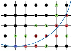
Figure 1.Discretization of a defect curve (blue). Red denotes the approximating lattice nodes.
3 Curved defect line
Let us consider a defect line as large as the lattice size. We would like to study if this line can change itself without breaking down. To characterize the resulting curves, we use a notion ofcurvature K: all the 2D curves form arcs of a certain radii with the constant length.
To begin with, we expect something like a collapse of the curved defect line due to the mutual attraction of the defects. A simple analytical analysis shows that average distance between points of an arc of a cirle increases with radius. Given that the defects are attracted to each other, we come to the conclusion that the curve tends to contract in a circle.
To form defect configurations, we need to convert a smooth curve to a discrete model that will allow us to identify the nodes occupied by defects. To do this, consider the followingnatural ap-proach. Assume that the radiusR ∈ Nof the arc is equal to an integer number of lengths of lattice constants. Fix initial node (node 0 in Figure1). Then two adjacent nodes (nodes 1) are considered and the distances from these nodes to the circle center are measured, so the node that provides the minimum of the deviation is selected:
min
j |rj−R|, j=1,2,
whererjis the distance discussed. Figure1demonstrates the successive steps of selecting sampling points, labeled with numbers from 1 to 8. The total amount of defects to be put in the lattice is determined by the line length.
Let us check the advantage of turning a line into an arc of a circle numerically. For this purpose, we choose lattices of several sizes and fill them with the discretized arcs of defects with different
radii. With the help of Monte Carlo simulation, the total energy of the system was calculated. All the computations were done at 1/T = 0.44. In paper [11] it is shown that critical temperature depends on defects’ concentration. However, as we consider curves of lengthL in lattices of size L2, the
concentration decreases as a function ofL. In such a situation, we neglect a small difference between
0.44, the critical temperature of pure lattice and the bulk critical temperature of the system considered. After we subtract the total energy of the configuration corresponding to a certain large radius (an immediate check showed that there is no difference, to do a subtraction with a straight line or with a
slightly curved arc). So, the energyE depicted in the figures of this Section equalsE = Etot(K)− Etot(K0),whereK0is a constant (rather small) curvature andEtot is the total energy (1).
(a) Energy per unit length of the curve as a function of the size of the lattice and curvature. A curve is as long as the lattice size. Attraction prevails, not counting the local repul-sion area. The reason for the effect is explained in the text. The solid line connecting data points is a B-Spline.
(b) The energy of a defect curve of fixed lengthL=75 for two lattice sizes: 75×75 and 150×150. The volume effect of repulsion is weakened. Data points are connected by line for clarity.
(c) Attraction between two curved lines arises then two ad-jacent endings become significant in perpendicular dimen-sion. Red arrow shows a part of the arc visible from the side of the other arc copy. A dashed line indicates a border with periodic boundary conditions.
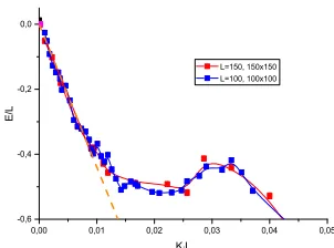
(d) Proof of scale invariance of the specific energyE/Lof the defective curve at 1/T=0.44. Both axes are dimension-less. B-Splines are used for clarity.
Figure 2.Curved defect line investigation.
significant, because the number of spin nodes between “semicircular branches” depends on the size of the lattice. At the same time, the graphs in Figure2a has a feature in behavior: there is a region of local maximum where the energy grows with the curvature.
An attentive reader will note that for line of lengthL=100 the maximal possible curvature (when
line is folded into a circle) is K=0.063, but Figure2a has a pointK=0,066...correspondingR=15.
This illustrates the problem of the discretization algorithm and the defect line put in lattice is not a perfect arc of a curcle at all.
Let’s analyze the curvature value K = 0.035 (where the curve rise in Figure2b starts) for the lattice 100×100. The radius corresponding to this curvature isR =1/K ≈28.571.A circle whose half-length isL1/2=100 has a diameterd=2L1/2/π≈63.662,which is approximately twice the size
(a) Energy per unit length of the curve as a function of the size of the lattice and curvature. A curve is as long as the lattice size. Attraction prevails, not counting the local repul-sion area. The reason for the effect is explained in the text. The solid line connecting data points is a B-Spline.
(b) The energy of a defect curve of fixed lengthL=75 for two lattice sizes: 75×75 and 150×150. The volume effect of repulsion is weakened. Data points are connected by line for clarity.
(c) Attraction between two curved lines arises then two ad-jacent endings become significant in perpendicular dimen-sion. Red arrow shows a part of the arc visible from the side of the other arc copy. A dashed line indicates a border with periodic boundary conditions.
(d) Proof of scale invariance of the specific energyE/Lof the defective curve at 1/T=0.44. Both axes are dimension-less. B-Splines are used for clarity.
Figure 2.Curved defect line investigation.
significant, because the number of spin nodes between “semicircular branches” depends on the size of the lattice. At the same time, the graphs in Figure2a has a feature in behavior: there is a region of local maximum where the energy grows with the curvature.
An attentive reader will note that for line of lengthL=100 the maximal possible curvature (when
line is folded into a circle) is K=0.063, but Figure2a has a pointK=0,066...correspondingR=15.
This illustrates the problem of the discretization algorithm and the defect line put in lattice is not a perfect arc of a curcle at all.
Let’s analyze the curvature value K = 0.035 (where the curve rise in Figure2b starts) for the lattice 100×100. The radius corresponding to this curvature isR =1/K ≈28.571.A circle whose half-length isL1/2=100 has a diameterd=2L1/2/π≈63.662,which is approximately twice the size
ofRmentioned above. This means that the curve with this curvature has the form of a semicircle.
Due to periodic boundary conditions, many identical copies of the defect curve are located in the system at a certain distance from each other. And they are attracted to each other. With further bending, the branches of each circle approach each other, but move away from the corresponding branches of adjacent curves. This increases the energy of the system. Consequently, the observed local maximum is avolume effect. Figure2c illustrates the phenomenon: in case of small K only
the endings themselves take part in the interaction, so few spins are involved in the process. But after the line is distorted, a lot more nodes appear opposite their counterparts, so energy volume effect is
tangible. Finally, as the curvature advances, the intensity of the effect decreases, and the attraction
again lowers the energy.
To overcome this problem, it would be good to move the neighboring curves far away from each other (to an infinite distance), but in a finite lattice model we can only try to double the size of the lattice. The length of the curve remains the same:L=75. The data obtained are shown in Figure2b.
The solid line has a local maximum (the region of repulsion of the branches), but the dashed line is almost monotonic and more adjacent to the linear approximation of the region of small curvature. In the second case, the neighboring curves interact less (due to the greater distance between them) and the attraction between the branches of one curve prevails.
To study the scale invariance, we have plotted the dimensionless productKLalong the horizontal axis (see Figure2d). The graphs coincide with remarkable accuracy. This supports the existence of scale invariance in the vicinity of the phase transition. It is important to note that the local maximum of the observed curves is an appearance of the volume effect. The study showed that when considering
large lattice, the linear energy’s dependence on curvature is strongly pronounced. According to the graphs presented in Figure2d, the coefficient of this dependence is defined:
E
L =aKL, a=−43,9±0,9. (3)
In case of an infinite lattice, if we bend a curve into a circle, an energy of 2πaper curve’s node is emitted (so far asL/R=2π). Thus, constantacan be treated with as a specific energy of a flat analog of a helix.
4 Defect-antidefect pair
The simplest deformation of the line is a tearing offone defect from it. Physically, an atom enters the
center of line, so that the defect migrates atom’s previous place (see Figure3a). As a result, we get one defect nearby the defect line and one occupied vacancy.
The process described is someway similar to production of particle-antiparticle pair in quantum field theory if we associate a defect torn from the line with a particle and the atom with an antiparticle. By means of this analogy, we treat the atom as an “antidefect”. The whole effect is called a
defect-antidefect pair production.
Above all, it is essential to create a pair from vacuum. If somebody affects the lattice in such a
way that a vacancy sinks in the second raw of lattice, two objects appear – a defect (vacancy in the depth) and an antidefect (the atom pushed into the fist layer). One can refer to defect line as a source of particles (the Dirac sea). It is well-known from experimental physics that energy is needed to bring a particle from the sea. So, we estimate an energetic threshold to appear. It is known that a pair of two particles undergo attraction. Will situation be the opposite this time? A numerical experiment casts light on the problem.
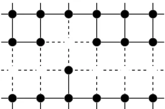
(a) Configuration corresponding to the moment of
a pair production. (b) One of configurations considered while energydependency of a pair interaction was studied. The distancedshown equals 2.
Figure 3.A process of defect-antidefect pair dispersing.
deal with two configurations: the first (black) is a straight line while the second (red) is implemented as shown in Figure3a. Apparently, correlation radius tends to zero at infinite temperature and defects stop to sense each other, so no significant difference is observed left-hand. However in solid form
(low temperatures) the diversity in configuration is appreciable. In this subsection we are interested in movement tendency that is how defect and antidefect had moved if they were loose. To arrive at a solution a series of configurations was tested with the object to energy variation. Thereby behaviour of the Ising model concerned with particle-antiparticle pair production coincides with that of field theory.
Meanwhile our study extends farther. Figure3b depicts a lattice, where defect and antidefect are separated by distanced=2. Let us examine interaction energy as a function ofd:
Eint(d)=EDA(d)−Ere f, (4)
whereEDA(d) is full energy of lattice with a defect-antidefect pair in distance ofd andEre f is the reference energy. The reference energy is the full energy of lattice with two defects fixed in some dis-tance between them. The reference energy is a level to calibrate the interaction effect. Theoretically,
the reference distance must be chosen as infinity, but we use a lattice approximation, so our field of activity is limited by the lattice size. The choice must be made so that two defects were far away from each other as soon as possible. Recalling that periodic boundary conditions are used, the distance can be a half of the lattice size.
The results of computer calculation (see Figure4b) reveal that the effect is appreciable enough. Eint(d) turns to be positive, so defect and antidefect tend to undergo mutual repulsion. It is an engaging effect: if somebody pushes an atom of lattice into a free space strip, then the vacancy, immersed into
the crystal, begins to run away from the initial position.
The results discussed are obtained using Monte Carlo on a 20×20 lattice. It is well-known that small lattices are prone to volume effects, so that results could be incorrect. To deal with the situation
in a proper way, we repeated the same calculation on a set of larger lattices and searched for an approximation. The process is shown in Figure4c. Is was proposed to lean on points far away from the critical point (we phase transition takes place). It is important, that peaks of all the four graphs fell onto the approximation line and drift slowly towards the critical point (0.44 in the graph). This is the cause, why we assume the intersection of the approximation line and vertical line of 1/Tcrto
(a) Configuration corresponding to the moment of a pair
production. (b) One of configurations considered while energy depen-dency of a pair interaction was studied. The distanced
shown equals 2.
(c) Defect-antidefect pair internal energy as a function of inversed temperature ford=0.
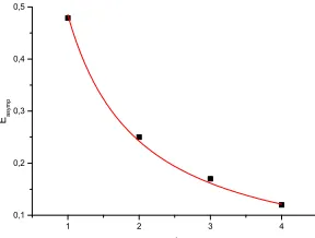
(d) Effective interation potencial vs. distance between the pair components. The Coulomb approximation could be ap-plied.
Figure 4.Defect-antidefect pair energy features.
be the volume limit (whereL → ∞). We call this valueEasymp that is the asymptotic energy of a defect-antidefect pair in an infinite lattice. It is a prediction though.
Next, the same prediction was made for other distances between pair components, so the asymp-totic interaction energy as a function of the distance is obtained (see Figure4d). Actually, the curve fits well the Coulomb potential, for which we get
Easymp(d)= a
d, a=0.485±0.006. (5)
5 Conclusion
We focus our intention on the problem of Casimir interaction of defects. To solve this problem we used the numerical Monte-Carlo simulation of Ising model with defects.
As a major goal, we studied the processes of defect line deformation. The simplest one is pulling-out the defect pulling-out of line with generation of “antidefect” (an atom appeared in the previous node of the defect). We confirmed that one should spend energy to create a pair. This process is the analogy to QFT’s process where a defect plays the role of a particle and defect line – of the Dirac sea. We showed that defect and antidefect undergo the forces of repulsion unlike the QFT. An analogy is given between the interaction of a pair with the electrostatic Coulomb interaction and a “charge” of a defect is obtained.
A study of the Casimir forces of interaction between extensive objects in spin models can help in studying the folding process of proteins. As a simplification, the entire variety of possible curves of fixed length was limited by curves of constant curvature. The one-parameter family of curves obtained in this way was investigated from the point of view of the most energetically favorable state. A tendency to radius decreasing is observed. Monte Carlo simulation showed that the reduction of the Casimir energy of such a line is proportional to its curvature.
6 Acknowledgements
The reported study was supported by the Supercomputing Center of Lomonosov Moscow State Uni-versity [13]. This work has been supported by the grant from the Russian Science Foundation (project number 16-12-10059).
References
[1] M.E. Fisher, P.G. de Gennes, Comptes rendus de l’Academie des sciences (Paris) Ser. B287, 207 (1978)
[2] M. Krech,The Casimir Effect in Critical Systems(1994)
[3] A. Gambassi, Journal of Physics: Conference Series161, 012037 (2009) [4] L.P. Kadanoff, Physics2, 263 (1966)
[5] M. Hasenbusch, Phys. Rev. E87, 022130 (2013)
[6] P. Nowakowski, A. Maciolek, S. Dietrich, Journal of Physics A: Mathematical and Theoretical
49, 485001 (2016)
[7] B.B. Machta, S.L. Veatch, J.P. Sethna, Phys. Rev. Lett.109, 138101 (2012) [8] G.M. Bell, Journal of Physics C: Solid State Physics5, 889 (1972)
[9] G.M. Bell, D.W. Salt, J. Chem. Soc., Faraday Trans. 272, 76 (1976)
[10] S.V. Titov, Y.K. Tovbin, Russian Journal of Physical Chemistry A85, 194 (2011) [11] T. Osawa, K. Sawada, Progress of Theoretical Physics49, 83 (1973)
[12] X. Wu, Y. Zhang, Phys. Rev. E92, 032108 (2015)