Parallel Event Selection on HPC Systems
MarcPaterno1,∗,JimKowalkowski1,∗∗, andSabaSehrish1,∗∗∗
1Fermi National Accelerator Laboratory, Batavia IL, USA
Abstract.In their recent measurement of the neutrino oscillation parameters, NOvA uses a sample of approximately 25 million reconstructed spills to search for electron-neutrino appearance events. These events are stored in an n-tuple format, in 250 thousand ROOT files. File sizes range from a few hundred KiB to a few MiB; the full dataset is approximately 1.4 TiB. These millions of events are reduced to a few tens of events by the application of strict event selection criteria, and then summarized by a handful of numbers each, which are used in the extraction of the neutrino oscillation parameters.
The NOvA event selection code is currently a serial C++program that reads
these n-tuples. The current table data format and organization and the selec-tion/reduction processing involved provides us with an opportunity to explore
alternate approaches to represent the data and implement the processing. We represent our n-tuple data in HDF5 format that is optimized for the HPC envi-ronment and which allows us to use the machine’s high-performance parallel I/O capabilities. We use MPI, numpy and h5py to implement our approach and
compare the performance with the existing approach. We study the performance implications of using thousands of small files of different sizes as compared
with one large file using HPC resources. This work has been done as part of the SciDAC project, “HEP analytics on HPC” in collaboration with the ASCR teams at ANL and LBNL.
1 The science problem
The NOvA collaboration has measured the parameters of the Pontecorva-Maki-Nakagaw-Sakata (PMNS) mixing matrix, which describes the transformation between the neutrino weak interaction eigenstates (νe,νµ,ντ) and the neutrino mass eigenstates (ν1,ν2,ν3). Their analysis consists of a search through millions of detector readouts periods—calledspills—to identify the small fraction of spills that contain neutrino interactions in the NOvA detector. The first part of their analysis involves the classification of candidate interactions, and the selection of
νµandνecharged current interaction candidates. The goal of the classification is to identify
and measure the relative frequency ofνeappearance events, which is the result of oscillations
of neutrinos in theνµbeam created at Fermilab.
2 The computing problem
The US Office of Science has been moving HEP towards the use of national infrastructure for scientific computing. The major computing centers consist of Argonne Leadership Computing Facility (ALCF), ORNL Leadership Computing Facility (OLCF), and National Energy Re-search Scientific Computing Center (NERSC). In the past, these very large-scale machines have been tailored for simulation applications utilizing fine-grained parallelism with success metrics that included FLOPS across the entire machine1. This has changed considerably with the current machines; they are much more focused on diverse workloads across many areas of science, and have been addressing issues of I/O performance and the processing of experimental data with distributed workflow2. The next generation of exascale machines will not only be much larger, but will also have heterogeneous computing elements to allow for artificial intelligence, data science, and large-scale computational workloads3. Measurements of success in using these machines will be more than just a port of existing applications to a new platform. Compute cycle providers will be looking for efficient use of the available resources: how well-utilized are the compute, network, memory, and I/O resources when they are used in a workflow or application; how much energy does it take to produce a result; how long does it take to compute the desired results?
Given the direction of HPC hardware and available compute cycles, our goal is to explore how we can use the capabilities and organization of these big machines to minimize the processing of analysis-level data, therefore greatly reducing the turnaround time to obtain physics results. As an example, with one million cores assigned to an analysis task, twenty-four million CPU hours can be applied to a problem in one day of running. Such an allocation is possible now when using all the cores on a node, and will be more straightforward in the near future. With such an allocation, analysis procedures that took more than a month can be delivered to a collaboration in less than one day. Analysis at this scale, with near real-time turn-around time, will make possible systematic studies and accuracy not possible before.
In order to address the desire for quicker turnaround given the ever-increasing data load and the need to effectively use new HPC resources, substantial modifications are necessary to both the (1) application structure and how data are organized and accessed, and (2) how workflows are constructed and orchestrated. The global parallel filesystems are the main connection to storage on all of the HPC systems. They are coupled to the computing infrastructure through the system interconnect, and permit high speed access to data from any compute node. The parallel nature of these filesystems allow for simultaneous coordinated access to the same file. The number of compute nodes is determined at batch submission time and allocated all at once. Integrating knowledge of data location into the application can allow complete dataset processing without the need of copying files and data across filesystems. Location information includes what part of the globally accessible data must be read and processed by what instance of the application across nodes allocated for this job. Careful sizing and structuring of data within files can allow for scaling application to any node count without performance loss due to I/O and communications overhead. We are moving analysis procedures towards this data-parallel approach to organizing applications. With this organization, workflow orchestration changes and becomes more tightly integrated into the application and the structure of the data. The scientific communities surrounding HPC have well-established software toolkits and libraries to effectively utilize the hardware available at HPC centers to solve problem at large scale. Over the past few years these tools have become more robust, more C++friendly, and can be used on modern Linux systems outside of the HPC facilities. Most relevant for
1https://www.top500.org/lists/2018/11/
2https://www.alcf.anl.gov/alcf-data-science-program 3https://www.exascaleproject.org/
this paper are HDF5 [1] for parallel I/O and MPI [2] for coordinating parallel applications. Additional abstractions that make data-parallel programming easy across processes, nodes, and threads, such as DIY [3] are also very important for HEP developers.
3 The traditional solution
In [4], NOvA reports on their work up to the date of publication, using a data sample corresponding to 8.85×10²⁰protons on target. This data sample contained about 25 million reconstructed beam spills, which are further divided into more than 500 millionslices, which are the atomic unit for NOvA analysis. These slices were searched for electron-neutrino appearance candidates. These data are stored in an n-tuple format in about 250 thousand ROOT4files. The typical file size is about 5.5 MiB; the full dataset is approximately 1.4 TiB. These hundreds of millions of slices were reduced to a few hundred candidate neutrino interactions by the application of strict selection criteria, and each was summarized by a handful of numbers, which are used in the extraction of the neutrino oscillation parameters.
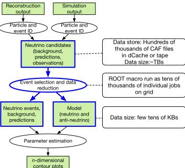
Figure 1 describes the analysis workflow as used by NOvA. As is traditional in HEP, this workflow is very strongly file-oriented. Parallel processing is achieved only at the file level, and a significant amount of bookkeeping work must be done to keep track of the large number of files being processed, as well as the many jobs used to process them.
Model (neutrino and anti-neutrino) Event selection and data
reduction Neutrino candidates (background, predictions, observations) Neutrino events, background, predictions Parameter estimation Reconstruction output Particle and event ID Simulation output Particle and event ID n-dimensional contour plots
Data store: Hundreds of thousands of CAF files
in dCache or tape Data size:~TBs
ROOT macro run as tens of thousands of individual jobs
on grid
Data size: few tens of KBs
Figure 1.The NOvA analysis workflow; boxes indicate data to be processed, ellipses indicate processing steps. The bold elements indicate the steps addressed in this work. The rounded rectan-gles on the right side show the traditional solution using thousands of small files.
CN CN CN CN
CN CN CN CN
CN CN CN CN
CN CN CN CN
srun -n 76800 shifter \ python process_nova.py novacaf.h5
High bandwidth global file system Login
Node
BB BB BB BB
Compute nodes connected Aries high-speed network novacaf.h5 striped High bandwidth burst buffers
Figure 2. This figure shows the HPC based ap-proach; a user interacts with the machine using login nodes, and is able to use the number of ranks specified with a singlesruncommand. The figure also shows how compute and IO nodes are organized in these machines, and how data are striped on a parallel file system.
Currently, the data are organized in CAF (Common Analysis Format) files, a ROOT format developed by NOvA for their analysis. In the CAF format, data for each slice is represented as a “StandardRecord” object. Each StandardRecord object contains several sub-objects, representing either summary information about the slice, or collections of “physics objects” (such as tracks and vertices) found in the slice. Thus, in this format, the reconstructed
information for each slice is represented as a tree structure, There are about 60 distinct classes in this data representation. Event selection in this form is done using a complex ROOT macro, which goes through slices serially, evaluating whether each slice isνµCC candidate, aνeCC
candidate, or is uninteresting. The ROOT macro implements on the order of 100 separate cuts. The hundreds of thousands of ROOT n-tuple files, each about 250 MiB in size and containing hundreds of spills, were processed by thousands of batch jobs run on available grid resources. The output is tens of KiBs of data describing the neutrino interaction candidates that is next used in the parameter estimation step. As the selection criteria were tuned on simulation samples, such processing was repeated many times. The processing of the actual 25 million event data sample on grid resources available to NOvA took several weeks.
4 The HPC solution
As discussed in section 2, we are now rethinking how code and data are organized to efficiently utilize the HPC machines. One goal is to minimize reading, i.e. only efficiently read portions of data that are needed by the analysis, and also to minimize communication and synchronization between processes to get the most data parallelism possible.
Our HPC-based solution uses an HDF5 format to store the data. It is organized into datasets (columns) and groups (tables) that is efficient for parallel IO and in-memory processing on HPC machines. MPI is used for multi-process parallelism along with the parallel IO features of HDF5. The cut functions (filter criteria) are implemented using Python, and make extensive use of pandas5and numpy6. We use mpi4py7and h5py8wrappers for MPI and HDF5.
Figure 2 shows the highest-level view of the HPC solution and environment. The single sruncommand shown in the figure 2 does the equivalent of launching 76800 batch jobs to process separate files. The HPC system consists of a huge number of multiprocessor nodes, with a high-bandwidth interconnect. The data are automatically staged from a huge global parallel filesystem to a high-bandwidth SSD array. NERSC’s Cori9supercomputer, for example, consists of two partitions: 2388 Intel Xeon “Haswell” nodes (32 cores each) and 9688 Intel Xeon Phi “Knights Landing” (KNL) nodes (68 cores each). All of these nodes use the same Cray “Aries” high-speed inter-node network (45 TB/s for KNL and 5.6 TB/s for Haswell). The Lustre scratch file system on Cori has 28 PB capacity (700 GB/s IO), and NVRAM “burst buffer” storage device (1.7 TB/s, 1.8 PB storage for staging). Cori is ranked as the 10th most powerful supercomputer in the world, as of June 2018.
4.1 Organization of data
As noted above, to make the data organization more amenable to data-parallel processing we mapped the tree-structured StandardRecord data into a set of tables. The resulting table structure contained approximately 80 tables, with the typical table containing about 20 columns. About half of the tables carry information that directly describes a single slice; such tables have exactly one entry per slice. These are referred to asregulartables. In the other tables, each row corresponds to some “physics object” (e.g.a track or a hit on a track). For these tables, there is a variable number of rows (from zero to many) carrying data relating to each slice. These tables are referred to here asirregular. Each table has one or more columns that provide the indexing information that allows us to make references between the data, for
5See https://pandas.pydata.org. 6See http://www.numpy.org.
7See https://bitbucket.org/mpi4py/mpi4py. 8See http://www.h5py.org.
information for each slice is represented as a tree structure, There are about 60 distinct classes in this data representation. Event selection in this form is done using a complex ROOT macro, which goes through slices serially, evaluating whether each slice isνµCC candidate, aνeCC
candidate, or is uninteresting. The ROOT macro implements on the order of 100 separate cuts. The hundreds of thousands of ROOT n-tuple files, each about 250 MiB in size and containing hundreds of spills, were processed by thousands of batch jobs run on available grid resources. The output is tens of KiBs of data describing the neutrino interaction candidates that is next used in the parameter estimation step. As the selection criteria were tuned on simulation samples, such processing was repeated many times. The processing of the actual 25 million event data sample on grid resources available to NOvA took several weeks.
4 The HPC solution
As discussed in section 2, we are now rethinking how code and data are organized to efficiently utilize the HPC machines. One goal is to minimize reading, i.e. only efficiently read portions of data that are needed by the analysis, and also to minimize communication and synchronization between processes to get the most data parallelism possible.
Our HPC-based solution uses an HDF5 format to store the data. It is organized into datasets (columns) and groups (tables) that is efficient for parallel IO and in-memory processing on HPC machines. MPI is used for multi-process parallelism along with the parallel IO features of HDF5. The cut functions (filter criteria) are implemented using Python, and make extensive use of pandas5and numpy6. We use mpi4py7and h5py8wrappers for MPI and HDF5.
Figure 2 shows the highest-level view of the HPC solution and environment. The single srun command shown in the figure 2 does the equivalent of launching 76800 batch jobs to process separate files. The HPC system consists of a huge number of multiprocessor nodes, with a high-bandwidth interconnect. The data are automatically staged from a huge global parallel filesystem to a high-bandwidth SSD array. NERSC’s Cori9supercomputer, for example, consists of two partitions: 2388 Intel Xeon “Haswell” nodes (32 cores each) and 9688 Intel Xeon Phi “Knights Landing” (KNL) nodes (68 cores each). All of these nodes use the same Cray “Aries” high-speed inter-node network (45 TB/s for KNL and 5.6 TB/s for Haswell). The Lustre scratch file system on Cori has 28 PB capacity (700 GB/s IO), and NVRAM “burst buffer” storage device (1.7 TB/s, 1.8 PB storage for staging). Cori is ranked as the 10th most powerful supercomputer in the world, as of June 2018.
4.1 Organization of data
As noted above, to make the data organization more amenable to data-parallel processing we mapped the tree-structured StandardRecord data into a set of tables. The resulting table structure contained approximately 80 tables, with the typical table containing about 20 columns. About half of the tables carry information that directly describes a single slice; such tables have exactly one entry per slice. These are referred to asregulartables. In the other tables, each row corresponds to some “physics object” (e.g.a track or a hit on a track). For these tables, there is a variable number of rows (from zero to many) carrying data relating to each slice. These tables are referred to here asirregular. Each table has one or more columns that provide the indexing information that allows us to make references between the data, for
5See https://pandas.pydata.org. 6See http://www.numpy.org.
7See https://bitbucket.org/mpi4py/mpi4py. 8See http://www.h5py.org.
9See http://www.nersc.gov/users/computational-systems/cori/.
example to know which hits are associated with a given track, and which tracks are associated with a given slice. Tables 1 and 2 show example table for each case. Such an organization allows for direct and efficient mapping of data to in-memory data structures.
We are exploring the appropriate size and number of files to use for this analysis. A single large file offers excellent scalability, as we have demonstrated with previous work. Either a single file or a number of moderately large (several hundred GiB) files can be striped across tens of OSTs (Lustre’s Object storage targets), which is critical for obtaining good performance from a global parallel filesystem. However, NOvA’s grid-based processing that creates the HDF5 files naturally creates hundreds of thousands of smaller files, and concatenation of these files requires additional processing time. A larger number of files increases the difficulty of obtaining optimal load balancing in the parallel processing. We will measure the speed of processing at several points of the continuum of possible file sizes to determine what is optimal. In order to use either a single large file or few large files, we are working on the performance evaluation of our concatenation program.
run subRun event slice distallpngtop ...35 more... 16433 61 356124 35 nan
16433 61 356124 36 -0.74013746 16433 61 356124 37 nan 16433 61 356125 1 nan 16433 61 356125 2 423.6337 16433 61 356125 3 -2.849864
Table 1.Organization of NOvA data records into regular table with one entry per neutrino slice.
run subRun event slice vtxid npng3d ...6 more... 16433 61 356124 35 0 0
16433 61 356124 36 0 1 16433 61 356124 36 1 1 16433 61 356125 36 2 5 16433 61 356125 1 0 1 16433 61 356125 3 0 0
Table 2.Organization of NOvA data records into irregular table with one entry per identified vertex in the interaction topology.
4.2 Reading and distributing information
vector that spans all the elements of our index columns (slices, events, subruns, and runs). The row index values above are the indices into those long vectors. The algorithm insures that no event is split between two ranks. An overview of the algorithm is as follows.
1. Each rank reads the index fields of the hdr table with one slice per row to calculate which events (and rows) ideally belong to it. All ranks use the same “fair share” function. 2. Each rank reads one row before and N rows after that ideal range in all tables to
determine if any events (or slices) are split. A rank will give up rows (up to N) at the beginning of its range to the “previous” rank, and take rows at the end (up to N) from the “next” rank to form a complete event.
3. At this point each rank has formed a portion of the global index map described above. The MPI “all gather” functions are used to exchange parts of the map with all ranks, with all ranks having the entire map for all tables. The map allows alignment of row reads by event ID (run, subrun, event) across all tables using rank ID.
4. Each rank uses the map to locate the full range of rows for each table that must be read. Figure 3 shows a simple view of the steps described above using four events and three ranks. The first table is a regular (one slice per row). There are twelve rows, and each rank is initially assigned four rows. Event ID information is inspected before and after to align row ranges on event boundaries. Rank 0 is assigned events one and two. Rank 1 assigned event three. Rank 2 assigned rows for event four. This mapping information is sent to all the ranks. A similar process is shown for the irregular table. Once the reading and data distribution is complete, each rank has its share from each table (pandas dataframe per table in memory).
sel_nuecosrej
rank 2
rank 0
rank 1
rank 2
rank 0
rank 1
rank 1
initial r
ead of index information
final event assignment for r
eading of physics data
vtx_elastic
rank 0
rank 2
rank 0
rank 1
rank 2
read of index information for irr
egular tables
final event assignment for r
eading of physics data
Figure 3.Blockwise organization of NOvA data into regular (left) and irregular (right) length records. This permits the indexing of information across different neutrino events (shown by different colors) and
the mapping of the data into the different ranks of the calculation.
4.3 Selection code
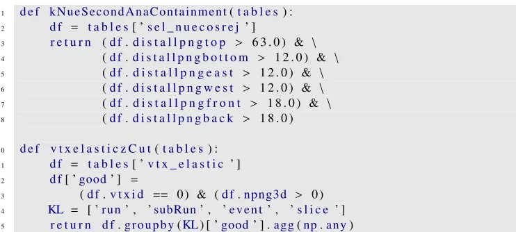
The selection code relies on the fact that the correct rows have been read by each rank, so that a given rank has access to all the information necessary to apply the selection criteria to all the slices for which that rank is responsible. Each of the selection criteria is implemented as a python function which accepts a dictionary of pandas dataframes, with a dataframe for each table the cut requires for its decision. Listing 1 shows an example of each of the two different kinds of selection functions. The functionkNueSecondAnaContainmentuses only the tablesel_nuecosrej, which is regular. Thus the comparisons made in the selection code are automatically vectorized (in the numpy sense)—a single comparison acts on all the slices
1 d e f kNueSecondAnaContainment(t a b l e s) :
2 d f = t a b l e s[ ’s e l _ n u e c o s r e j ’ ]
3 r e t u r n (d f.d i s t a l l p n g t o p > 6 3 . 0 ) & \
4 (d f.d i s t a l l p n g b o t t o m > 1 2 . 0 ) & \
5 (d f.d i s t a l l p n g e a s t > 1 2 . 0 ) & \
6 (d f.d i s t a l l p n g w e s t > 1 2 . 0 ) & \
7 (d f.d i s t a l l p n g f r o n t > 1 8 . 0 ) & \
8 (d f.d i s t a l l p n g b a c k > 1 8 . 0 )
10 d e f v t x e l a s t i c z C u t(t a b l e s) : 11 d f = t a b l e s[ ’v t x _ e l a s t i c ’ ]
12 d f[ ’good’ ] =
13 (d f.v t x i d == 0 ) & (d f.npng3d > 0 )
14 KL = [ ’run’ , ’subRun’ , ’event’ , ’s l i c e ’ ]
15 r e t u r n d f.groupby(KL) [ ’good’ ] .agg(np.any)
Listing 1.Example analysis code demonstrating part of the selection of neutrino candidates.
represented in the dataframe with no explicit loop in the Python code. This function returns a numpy array of logical values, one for each slice represented in the dataframe. The second function in the listing,vtxelasticzCut, acts on an irregular table,vtx_elastic. Since a decision is desired for each slice, the pandasgroupbyfunction is used to produce a single answer (from the aggregation functionnp.any). This will return a value of True for each slice that contains any good vertex. Omitted (for reasons of space) is the code that is used to combine the results of different cuts for each slice, to yield a single answer for each slice.
We think it is important to note that this code, while written in the same fashion as serial code, is implicitly data-parallel. Users are not required to learn parallel code/programming for these tasks. Furthermore, we can rely upon the implementation of numpy deployed on the HPC machine to make use of vectorized CPU instructions available on that machine, and so our code is both portable and efficient.
5 Workflow for translating old style data to the new style
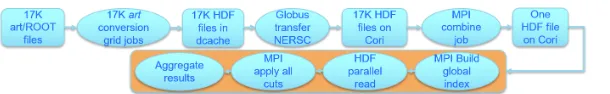
We have developed a workflow process to translate the traditional data format and organization to the new style data in HDF5. We have used theartframework [5]10to write these HDF5 files. We have written anartmodule, HDFMaker, to be used in the NOvA workflow that also creates the CAF files. This module writes one HDF5 tabular file (described above) per job. The job is run on the Fermi grid nodes and one small HDF5 file corresponding to eachart-ROOT input file is generated. This results in thousands of small HDF5 files. For testing our workflow, we currently have a sample of 17 thousand files. Using the Globus transfer service between Fermilab and NERSC, we transferred all of these files to NERSC. As described earlier, we are currently working on the evaluation of the production and processing of either one (or a few) large HDF5 files, or of many small files. Figure 4 shows all of these steps in the workflow. The “MPI combine job” is the (possible) concatenation step. The yellow box with the last four ellipses represents data processing phase; that has been described in detail in section 4.
6 Summary and conclusion and future work
The program design and data restructuring described here has primarily focused on addressing improvements identified in section 2. After all cut functions have been implemented and
Figure 4.Workflow for translating old-style data to new-style data.
verified, we will work on scaling tests and optimization improvements. We have benchmark results for HDF5 I/O on NERSC Cori from an earlier LArIAT/LArSoft demonstration that
indicate what we should expect from this system; we were able to show perfect scaling up to 76,800 ranks (individual processes on cores), with reading and decompressing of 42TB of waveform data in under 20 seconds of wall-clock time. The traditional NOvA event selection ROOT application will be used as a baseline for performance studies at both ALCF and NERSC. A data-parallel C++-MPI application using DIY, HDF5, and Eigen will also be
implemented to have a performance comparison with the Python version.
An important outcome of this work is that NOvA has already taken ownership of theart module HDFMaker. The conversion tools will be extracting data from NOvA into HDF5 for deep network training with Tensorflow and other mainstream machine-learning toolkits.
As part of our SciDAC411 project, the next steps will be to address larger workflow problems, where we will study event selection choices to evaluate systematic uncertainties in the mixing parameter measurements. The low latency, near real-time processing that is available at large scale enables these types of studies.
7 Acknowledgments
We would like to thank the members of the NOvA collaboration for providing us with the relevant material for this work. This manuscript has been authored by Fermi Research Alliance, LLC under Contract No. DE-AC02-07CH11359 with the U.S. Department of Energy, Office of
Science, Office of High Energy Physics. This material is based upon work supported by the U.S.
Department of Energy, Office of Science, Office of Advanced Scientific Computing Research,
Scientific Discovery through Advanced Computing (SciDAC) program. This research used resources of the National Energy Research Scientific Computing Center, a DOE Office of
Science User Facility supported by the Office of Science of the U.S. Department of Energy
under Contract No. DE-AC02-05CH11231.
References
[1] The HDF Group,Hierarchical Data Format, ver. 5(1997-2018),http://hdfgroup.org [2] The MPI Forum, MPI: A Message-Passing Interfacer Standard, version 3.1 (2015),
http://www.mpi-forum.org
[3] T. Peterka, R. Ross, W. Kendall, A. Gyulassy, V. Pascucci, H.W. Shen, T.Y. Lee, A. Chaud-huri,Scalable Parallel Building Blocks for Custom Data Analysis, inProceedings of Large Data Analysis and Visualization Symposium LDAV’11(Providence, RI, 2011)
[4] P. Adamson, L. Aliaga, D. Ambrose, N. Anfimov, A. Antoshkin, E. Arrieta-Diaz, K. Aug-sten, A. Aurisano, C. Backhouse, M. Baird et al., Physical Review Letters118, 231801 (2017)
[5] C. Green, J. Kowalkowski, M. Paterno, M. Fischler, L. Garren, Q. Lu, J. Phys. Conf. Ser. 396, 022020 (2012)