R E S E A R C H
Open Access
An incremental learning algorithm for the
hybrid RBF-BP network classifier
Hui Wen, Weixin Xie, Jihong Pei
*and Lixin Guan
Abstract
This paper presents an incremental learning algorithm for the hybrid RBF-BP (ILRBF-BP) network classifier. A potential function is introduced to the training sample space in space mapping stage, and an incremental learning method for the construction of RBF hidden neurons is proposed. The proposed method can incrementally generate RBF hidden neurons and effectively estimate the center and number of RBF hidden neurons by determining the density of different regions in the training sample space. A hybrid RBF-BP network architecture is designed to train the output weights. The output of the original RBF hidden layer is processed and connected with a multilayer perceptron (MLP) network; then, a back propagation (BP) algorithm is used to update the MLP weights. The RBF hidden neurons are used for nonlinear kernel mapping and the BP network is then used for nonlinear classification, which improves classification performance further. The ILRBF-BP algorithm is compared with other algorithms in artificial data sets and UCI data sets, and the experiments demonstrate the superiority of the proposed algorithm.
Keywords:Radial basis function (RBF), Back propagation (BP), Incremental learning, Hybrid, Neural network
1 Introduction
In the field of pattern recognition and data mining, various methods and models are proposed to solve different problems. Existing methods can be divided into two levels including data level and algorithmic level. The data levels are mainly concerned with vari-ous sampling techniques [1]. The algorithmic level tried to apply or improve varieties of existing trad-itional learning algorithms such as fuzzy clustering
[2], Markovian jumping system [3–5], k-nearest
neighbors [6], and neural network, where single-layer feed-forward networks (SLFNs) have been intensively studied in the past several decades and applied to solve various problems in different fields, such as image recognition [7], signal processing [8], disease prediction [9], and industrial fault diagnosis [10]; in particular, radial basis function (RBF) neural networks offer an effective mechanism for nonlinear mapping and classification. In a typical RBF network, the num-ber of hidden neurons is assigned a priori [11, 12], which leads to poor adaptability for different sample sets. Several sequential learning algorithms have been
proposed to determine proper sizes of RBF network architectures. A resource allocation network (RAN) for constructing the RBF network is proposed in [13], which uses the novelty of incoming data as the learn-ing strategy. A RAN algorithm based on an extended Kalman filter (RANEKF) is proposed in [14], which uses the extended Kalman filter algorithm instead of the least mean squares (LMS) algorithm. In [15], a minimal resource allocation network (MRAN) is pro-posed, which is allowed for the deletion of the previ-ous center. The deletion strategy is based on the overall contribution of each hidden unit to the net-work output. A sequential learning algorithm for growing and pruning the RBF (GAP-RBF) is proposed in [16, 17]; this algorithm uses the significance of neurons as the learning strategy. In [18], a Gaussian mixture model (GMM) to approximate the general-ized growing and pruning evaluation formula is pro-posed; the GMM can be used for problems with a high-dimensional probability density distribution. In [19], an error correction (ErrCor) algorithm is used
for function approximation; this algorithm can
achieve a desired error rate with fewer RBF units. Other methods have also been established to identify
* Correspondence:[email protected]
ATR Key Lab of National Defense, Shenzhen University, 518060 Shenzhen, China
a proper architecture while maintaining a desired accuracy [20–22].
Support vector machines (SVMs), which are max-imal margin classifiers, can also be used to train SLFNs. RBFs and SVMs differ in that at the output layer, a SVM employs convex optimization to find an optimal linear classifier, whereas the output weights of RBF network are typically estimated by a linear least squares algorithm, such as the LMS or recursive least squares (RLS) algorithm. Regarding other train-ing SLFNs, extreme learntrain-ing machines (ELMs) are proposed in [23]; ELMs choose random hidden neuron parameters and calculate the output weights with the least squares algorithm. This method can achieve a fast training speed. Subsequently, an online sequence extreme learning machine (OS-ELM) algo-rithm that can learn one by one and data blocks of the input samples is proposed in [24]. In ELMs, the number of hidden nodes is assigned a priori, and
many nonoptimal nodes may exist; thus, in [25–28],
several types of growing and pruning techniques based on ELMs are proposed to effectively estimate the number of hidden neurons.
All of the algorithms for training SLFNs consist of two stages: (1) suitable feature mapping and (2) out-put weight adjustment. To train SLFNs efficiently, in this paper, a potential function is introduced in the feature mapping stage to train the sample space, and an incremental learning method of constructing RBF hidden neurons is proposed. Note that although the sequence learning RBF algorithms can also generate RBF hidden neurons automatically, because of the lack of global information in the sample space, the adaptability of complex sample space may be poor. In contrast to GAP-RBF, the proposed method does not require an assumption that the input samples obey a unified distribution. Furthermore, it does not need to fit the input sample distribution, such as the algo-rithm proposed in [18]. The proposed method utilizes global information about each class of training sample space and can generate RBF hidden neurons incre-mentally to adapt the sample space. By using a poten-tial function to measure the density in each class of training sample space, the corresponding RBF hidden neurons that cover different sample areas can be established. The center of the Gaussian kernel func-tion can be determined by learning the density of dif-ferent regions in the training sample space. Once the width is given, a hidden neuron is generated and in-troduced into the RBF network, and a mechanism for eliminating the potentials of original samples is pre-sented. This mechanism is ready for the next learning step, and thus, the RBF centers and number of hid-den neurons can be effectively estimated. In this way,
a suitable network size for RBF hidden layer that matches the complexity of the sample space can be built up. Thus, the proposed method solves the prob-lem of dimension change from sample space mapping to feature space, and it reduces the restrictions on the sample sets, which is adaptable to more complex sample sets.
In this paper, a hybrid RBF-BP network architecture is designed for the output weight adjustment stage to further improve the generalization and classification performance. The output of the original RBF hidden layer is processed and connected with a new hidden layer, which means that the output of the original RBF hidden layer, the new hidden layer, and the out-put layer consists of a multilayer perceptrons (MLPs), and the output of the original RBF hidden layer is the input of the MLPs. Once the network architecture is established, a back propagation (BP) algorithm is used to update the weights of the MLPs. In the hybrid RBF-BP network, the RBF hidden neurons are used for nonlinear kernel mapping, the complexity of sample space is mapped onto the dimension of the BP network input layer, and the BP network is then used for nonlinear classification. The nonlinear kernel mapping can improve the separability of sample spaces, and a nonlinear BP classifier can then supply a better classification surface. In this manner, the
im-proved network architecture combines the local
response characteristics of the RBF network with the global response characteristics of the BP network, which simplifies the neuron number selection in the BP network hidden layer while further reducing the dependence on space mapping in the RBF hidden layer.
algorithm. The results indicate that the ILRBF-BP al-gorithm can provide a higher classification accuracy with comparable complexity.
The remainder of this paper is organized as follows. Section 2 describes the principal ideas of the ILRBF-BP, followed by a summary of the algorithm. Section 3 presents the experimental results and performance comparisons with other existing batch and sequential algorithms. Section 4 provides the conclusions of this study.
2 Main concepts of the ILRBF-BP algorithm
In this section, the main concepts of the ILRBF-BP algorithm are described. First, we provide the problem definition of the basic RBF network and then present the incremental learning algorithm for constructing RBF hidden neurons. Then, a hybrid RBF-BP network architecture is designed, and the ILRBF-BP algorithm is summarized. Finally, a method of adjusting the out-put saturation for multi-class classification problem is proposed.
2.1 Problem definition
For a RBF network, the output can be given by
FðxÞ ¼X is the response of the kth hidden node for an input vector x, where x∈Rt; ωk is its connecting weight to the output node, which determines the classification surface; and μk and σk are the center and width of the kth hidden node, respectively, where k= 1, 2,…K.
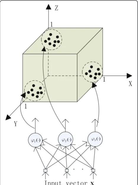
A RBF network can localize the input sample space, which maps input samples to the interior of the hypercube, and the localized area is near a vertex. The dimension of the hypercube is the number of RBF hidden neurons. Thus, when going through the
RBF network, an input vector x∈Rt can be denoted
as f:Rt→(0, 1]K. Figure 1 shows the results of map-ping input samples going through the RBF hidden neurons, where the number of RBF hidden neurons is
set as K= 3. In Fig. 1, we assume that every input
sample vector is near the center of a RBF hidden neuron and that there is no overlap area covered by different RBF hidden neurons.
Figure 1 illustrates that in a RBF network, to achieve good training algorithms, an effective method
of mapping the input sample space should be estab-lished, which means completing the estimation of the parameter set fK;μk;σkgKk¼1. Then, an effective classi-fication surface is needed, which depends on output weight adjustment.
2.2 Incremental learning algorithm for constructing RBF hidden neurons
In the fields of data mining and pattern recognition, potential functions can be used for density clustering and image segmentation (IS) [30]. Several methods of constructing potential function are proposed in [31]; here, we choose the potential function
γðx1;x2Þ ¼ 1 1þT⋅d2ðx1;x2Þ
ð3Þ
where γ(x1,x2) represents the interaction potential of
two points x1,x2 in the input sample space, d(x1,x2)
represents the distance measure, and T is a constant, which can be regarded as the distance weighting factor.
Given a training sample set S, where a specific label
yi,yi∈{yi;i= 1, 2,…h} is attached to each sample vectorx
inS,his the number of pattern class. LetSidenote the set
of feature vectors that are labeledyi,Si¼ fxi1;xi2;…;xiNig, whereNiis the number of training samples in theith
pat-tern class. Thus,S¼∪h
Letxivbe the baseline sample; then, the interaction po-tential of all other samples toxivcan be denoted as
ρðxi
Therefore, the potentials of each sample in Si is
given by
The potentials can be used to measure the density of different regions in the pattern class. Potentials are relatively large in the dense region, whereas they are relatively small in the sparse region. Once the
poten-tials of each sample in Si are given, the sample with
the maximum potential can be selected, where it is assumed the sample is xip, that is,
In a RBF network, the activation response of hidden neurons has local characteristics. The sample space is divided into different subspaces by establishing differ-ent Gaussian kernel functions. To generate valid Gaussian kernel functions, we find the most densely region in the sample space and then establish a Gaussian kernel to cover the region. For that purpose, the sample with the maximum potential is chosen as the center of Gauss kernel function, which is given below.
μk ¼xip ð8Þ
where k refers to the number of RBF hidden neurons generated. To simplify the calculation, the width is fixed and selected by cross validation.
When a hidden neuron is established, it is necessary to eliminate the potentials of the region to find the next center in the remaining samples. This process can be updated by
where xip is the center of the current hidden neuron. For the potential value update process, Eq.(9) shows when a sample xiv is close to the centerxip, the poten-tial value of xiv is attenuated fast, whereas when a sample xiv is far away from the center, the potential value of xiv is attenuated slowly. When meeting the inequality
max ρnew xi1 ;ρnew xi2 ;…;ρnew xiNi
n o
>δ ð10Þ
a new hidden neuron is introduced into the RBF net-work and is ready to search for the next center; other-wise, the algorithm of constructing RBF hidden neurons
in the current pattern class is over, where δ is a
threshold.
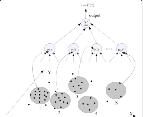
The above process is called the incremental learning algorithm of constructing RBF hidden neurons. Figure 2 shows a schematic diagram of generating RBF hidden neurons incrementally, where the serial numbers in the training sample space represent the regions covered by different RBF hidden neurons. These covered regions transition from dense to sparse. The incremental learn-ing algorithm of constructlearn-ing RBF hidden neurons is summarized in Algorithm 1.
2.3 Hybrid RBF-BP network architecture
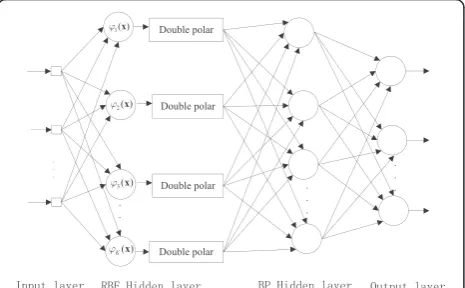
As noted above, in a typical RBF network, the output weights are typically estimated by a linear least squares algorithm, such as the LMS or RLS algorithm. In this section, we transform the linear least squares algorithm into a nonlinear algorithm. When classifying a problem, a nonlinear algorithm can supply a better classification surface to adapt the sample space. For that purpose, a hybrid RBF-BP network architecture is designed. The output of the RBF hidden neurons is processed and con-nected with a MLPs network, and then, the nonlinear BP algorithm is used to update the weights of the MLPs. The architecture of the hybrid RBF-BP network is shown in Fig. 3, which consists of four components:
1. The input layer, which consists oftsource nodes, wheretis the dimensionality of the input vector
2. The RBF hidden layer, which consists of a group of Gaussian kernel functions:
φkð Þ ¼x exp −
1 2σ2
k
jjx−μkjj2
; k¼1;2;…K ð11Þ
where μk and σk are the center and width of the hidden neuron, respectively, and K is the number of hidden neurons.
3. The BP hidden layer, which consists of the neurons between the RBF hidden layer and output layer. The induced local fieldvð Þjl for neuronjin layerlof the BP network is
vð Þjl ¼X i
ωð Þl jiy
l−1
ð Þ
i ð12Þ
whereyðil−1Þis the output signal of the neuroniin the pre-vious layerl-1 of the BP network andωð Þjil is the synaptic weight of neuron jin layerl that is fed from neuroniin layerl-1. Assuming the use of a sigmoid function, the out-put signal of neuronjin layerlis
yð Þjl ¼φj vj ¼atanh bvj ð13Þ
whereaandbare constants.
If neuron jis in the first BP network hidden layer, i.e., l= 1, set
yð Þj0 ¼gjð Þx ð14Þ
where gj(x) is the double polar output of φj(x) and can be denoted as
gjð Þ ¼x 2⋅φjð Þx −1 ð15Þ
4. The output layer. SetLis the depth of the BP network, note the depth of the BP network is equal to the sum of the BP network input layer, the hidden layer, and the output layer, i.e., ifl= 1, thenL= 3, and the output can be given as
oj¼yL ð Þ
j ð16Þ
In Fig. 3, the double polar processing can ensure the val-idity of the BP network input. The hybrid RBF-BP net-work architecture is designed such that the RBF netnet-work has good stability, where the activation response in the RBF hidden neurons has local characteristics and maps the output value between 0 and 1. Thus, the original sam-ples including outliers will be limited to a finite space. When the results of mapping the RBF hidden neurons are
processed and used for the input of the BP network, the convergence rate of the BP algorithm can be increased and local minima can be avoided. For a BP network, the activation response in hidden neurons has global charac-teristics, especially those regions not fully displayed in the training set. Therefore, the hybrid RBF-BP network archi-tecture is a reasonable model; it provides a new strategy that combines the local characteristics of the RBF network with the global characteristics of the BP network. In addition, the hybrid network simplifies the number of neurons in the BP hidden layer while further reducing the dependence on space mapping in the RBF hidden layer.
A single hidden layer MLP neural network with an input-output mapping can provide an approximate realization of any continuous mapping [32]. Combined with the above discussion, in the hybrid network, we set the number of BP network hidden layers asl= 1.
2.4 Adjustment of the output label values
The ILRBF-BP algorithm can handle binary problems and multi-class problems. For multi-class classifica-tion problems, suppose that the observaclassifica-tion data set is given as fxn;yngNn¼1, where xn∈Rt is an t‐
dimen-sional observation features and yn∈Rh is its coded
class label. Here, h is the total number of classes,
which is equal to the number of output hidden
neu-rons. If the observation data xn is assigned to the
class label c, then the cth element of yn= [y1,…,yc,
…yh]T is 1 and other elements are −1, which can be
denoted as follows:
yj¼ −1 if j¼c
1 otherwisej¼1;2;…;h
ð17Þ
The output tags of the ILRBF-BP classier areŷn= [ŷ1,
…,ŷc,…ŷh]T, where
^yj¼ sgn oj ; j¼1;2;…h ð18Þ
According to the coding rules, only one output tag value is 1 and the other value is −1. If this condition is not met, the output tag is saturated and must be adjusted. Therefore, we set an effective way to
correct the saturation problem in the learning
process, which can be denoted as the pseudo code in Algorithm 3.
3 Performance evaluation of the ILRBF-BP algorithm
In this section, we evaluate the performance of the ILRBF-BP algorithm using two artificial classification problems from [33] and three classification problems from the UCI machine learning repository [34]. The arti-ficial binary data sets, including the Double-moon and Twist problems are used to measure the unique features of ILRBF-BP and the main advantages of the results over others. Table 1 provides a description of the classifying data sets, where Double-moon, Twist, and IS are well-balanced data sets and Heart and vehicle classification (VC) are imbalanced data sets. For balanced data sets, the numbers of training samples in each class are identi-cal. For the heart problem, the numbers of training sam-ples in classes 1 and 2 are 33 and 40, respectively. For the VC problem, the numbers of training samples in classes 1–4 are 119, 118, 98, and 89, respectively.
3.1 Performance measures
In this paper, the overall and average per-class classifica-tion accuracies are used to measure performance. The confusion matrix Q is used to obtain the class-level per-formance and global perper-formance of the various classi-fiers. Class-level performance is measured by the percentage classification (ηi), which is defined as
ηi¼ qii
NTi ð19Þ
where qii is the number of correctly classified samples and NTi is the number of samples for the class yi in the training/testing data set. The overall (ηo) and average per-class (ηa) classification accuracies are defined as
ηo¼100
1
NT
Xh i¼1
qii ð20Þ
ηa ¼100
1
h
Xh i¼1
ηi ð21Þ
wherehis the number of classes and NTis the number of training/testing samples.
3.2 Performance comparison
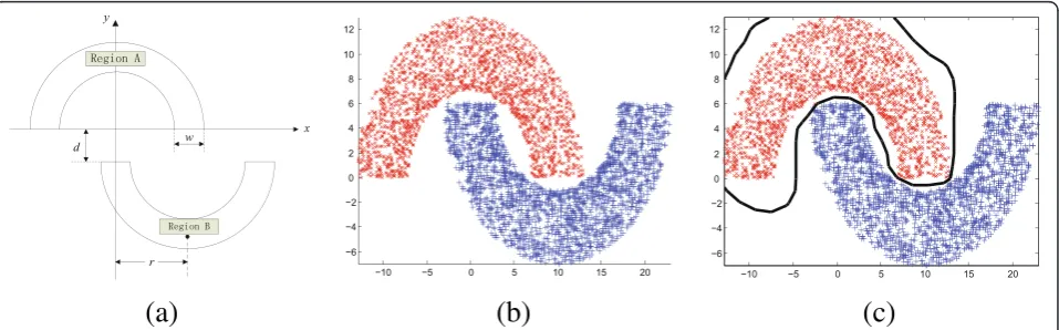
3.2.1 Artificial binary data sets: Double-moon problem The prototype and data set of the Double-moon classifi-cation problem are shown in Fig. 4a, b, respectively,
where r= 10, ω= 6 and d=−6. The main parameters
of distance weighting factor, width, incremental
learning threshold, number of BP hidden neurons,
and momentum constant in ILRBF-BP are set as T=
1, σ= 3, δ= 0.01, M= 5, and α= 0, respectively. Fig-ure 4c shows the classification results for the testing samples under these parameters. The classification results illustrate that the proposed algorithm can provide a superior classification surface. Figure 5 shows using different width parameters to cover the training sample space, where each cover generates a RBF hidden neuron and the number of RBF hidden neurons is increased incrementally, the bold lines represent the first coverage region in each pattern class. In Fig. 5, with the increase of the width param-eter, the corresponding region covered each RBF hid-den neuron is increased accordingly, which will affect the location of the next center, thus generates differ-ent RBF hidden neurons. Though the number of RBF hidden neurons has changed, ILRBF-BP still can effectively cover each class of training samples. Thus, the incremental learning algorithm based on potential function clustering is feasible. ILRBF-BP can be well adapted to the sample space, which is an effective algorithm to incrementally generate RBF hidden neu-rons for the Double-moon problem.
Figure 6a, b demonstrates that when the number of training samples has changed, KMRBF-BP needs less
(a)
(b)
(c)
Fig. 4aDouble-moon classification problem.bDouble-moon data set.cClassification result of the ILRBF-BP algorithm
Table 1Descriptions of the classifying data sets
Data sets No. of features No. of classes No. of training No. of testing Attribute Sources
Double-moon 2 2 200~2000 4000 Balance Artificial
Twist 2 2 200~2000 4000 Balance Artificial
Heart 13 2 73 230 Imbalance UCI
IS 19 7 210 2100 Balance UCI
number of RBF hidden neurons than KM-RBF. When the number of training samples is more than 500, KMRBF-BP can get a higher classifying accuracy than KM-RBF. These results show that the hybrid RBF-BP network architecture is effective, which can improve the classifying accuracy and reduce the dependence on the original sample space mapping. In GAP-RBF and ILRBF-BP, the number of RBF hidden neurons is generated automatically. ILRBF-BP needs less number of RBF hid-den neurons than GAP-RBF, and the overall testing ac-curacy outperforms GAP-RBF. The classifying acac-curacy of ILRBF-BP is comparable with SVM and KMRBF-BP and outperforms ELM and KM-RBF. Note that the num-ber of KM-RBF and KMRBF-BP is selected manually. When changing the number of hidden neurons several times, the one with the highest overall testing accuracy is selected as the suitable number of hidden neurons. As ILRBF-BP utilizes global information about each class of training sample space, it can generate RBF hidden neu-rons incrementally to adapt the sample space, and the hybrid RBF-BP network architecture improves the net-work performance further.
3.2.2 Artificial binary data sets: Twist problem
The prototype and data set for the twist classification problem are shown in Fig. 7a, b, respectively, whered1
= 0.2, d2= 0.5 and d3= 0.8. Compared to the
Double-moon problem, the twist classification problem is more complex and can thus be used to evaluate the classifica-tion performance of the different algorithms. The main parameters of distance weighting factor, width, incre-mental learning threshold, number of BP hidden
neu-rons, and momentum constant in ILRBF-BP are set asT
= 200, σ= 0.15, δ= 0.01, M= 5, and α= 0, respectively. Figure 7c shows the classification results for the testing samples under these parameters. The classification re-sults illustrate that the proposed algorithm still provides a superior classification surface for the Twist classifica-tion problem. Figure 8 shows using different width pa-rameters to cover the training sample space, where each cover generates a RBF hidden neuron. In Fig. 8, the bold lines represent the first coverage region, which denote the most dense region in each pattern class. Although there are some overlap in different coverage regions, ILRBF-BP still can effectively cover each class of training
(a)
(b)
(c)
Fig. 5Using different width parameters to cover the training sample space for Double-moon classification problem.aσ= 2.bσ= 3.cσ= 4
(a)
(b)
samples and generate corresponding RBF hidden neu-rons incrementally.
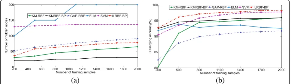
Figure 9a, b demonstrates that when the number of training samples has changed, KMRBF-BP needs less number of RBF hidden neurons than KM-RBF and can get a higher classifying accuracy. Thus, the hybrid RBF-BP network architecture improves the classifying accuracy and reduces the dependence on the original sample space mapping. Note that in KM-RBF and KMRBF-BP, when the number of training samples is changed, the number of RBF hidden neurons has to be adjusted manually; other-wise, it will lead to a poor classification accuracy. Com-pared to KM-RBF and KMRBF-BP, ILRBF-BP can adapt the training sample space well; when the number of train-ing samples is changed, the number of RBF hidden neu-rons in ILRBF-BP is changed accordingly and can get a higher classifying accuracy. Compared to GAP-RBF, ILRBF-BP can better adapt to the change of sample space. The classifying accuracy of ILRBF-BP outperforms GAP-RBF as well as SVM and ELM. Thus, the incremental learning algorithm based on potential function is effective, which utilizes global information about each class of
training sample space to construct RBF hidden neurons incrementally, and the hybrid RBF-BP network architec-ture improves the network performance further.
3.2.3 UCI binary data set: Heart problem
In this section, the Heart problem in the UCI binary data set is used to evaluate the performance of the ILRBF-BP algorithm. In the Heart problem, the sample distribution values of each dimension are between 0 and 1, and the main parameters of distance weighting factor, width, incremental learning threshold, number of BP hidden neurons, and momentum constant in ILRBF-BP are set as T= 1, σ= 1.2, δ= 0.001, M= 5, and α= 0.1, respectively. As noted above, the Heart problem is an imbalanced classification problem. This, in addition to the overall testing ηo, the average testingηais also used
to measure the performance of each algorithm.
The performance comparisons between ILRBF-BP and the other batch learning algorithms are shown in Table 2. For the Heart problem, the overall and average testing accuracy of ILRBF-BP are clearly higher than those of SGBP, and the proposed algorithm outperforms ELM
(a)
(b)
(c)
Fig. 8Using different width parameters to cover the training sample space for the twist classification problem.aσ= 0.1.bσ= 0.15.cσ= 0.2
(a)
(b)
(c)
and KM-RBF by approximately 2.5–5 %. The average testing accuracy of ILRBF-BP is 1.74 % lower than that of the SVM; however, the overall testing accuracy is ap-proximately 3 % higher than that of the SVM, and fewer hidden neurons are needed.
3.2.4 UCI multi-class data sets: IS and VC problems
In this section, the IS and VC problems are used to evaluate the performance of the ILRBF-BP algorithm. The output saturation is adjusted for the multi-class classifying problem in the ILRBF-BP algorithm. For the IS problem, the sample distribution range in each dimension is different, so the inputs of each algo-rithm are scaled appropriately between 0 and +1. The main parameters of distance weighting factor, width, incremental learning threshold, number of BP hidden neurons, and momentum constant in ILRBF-BP are
set as T= 1, σ= 0.3, δ= 0.001, M= 8, and α= 0.2,
respectively. The IS problem is a well-balanced data set; the number of training samples in each class is
30, and the overall testing ηo is used to measure the
performance of each algorithm. For the VC problem, the sample distribution values of each dimension are
between −1 and +1, and the main parameters of
distance weighting factor, width, incremental learning
threshold, number of BP hidden neurons, and
momentum constant in ILRBF-BP are set asT= 1, σ=
0.4, δ= 0.001, M= 9, and α= 0.1, respectively. The
number of training samples in each class is 119, 118, 98, and 89. The VC problem is a highly imbalanced data set, where the strong overlap between the classes influences the performance of each algorithm. The
overall testing ηo and average testing ηa are used to
measure the performance of each algorithm.
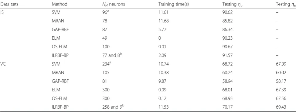
Table 3 shows the performance comparisons for the IS and VC problems. For the IS problem, the overall testing
accuracy of ILRBF-BP is approximately 5–6 % higher
than those of MRAN and GAP-RBF and approximately
0.9–1.3 % higher than those of OS-ELM, SVM, and
ELM. For the VC problem, the overall and average
test-ing accuracies of ILRBF-BP are approximately 9–11 %
higher than those of MRAN and GAP-RBF and
approxi-mately 1.2–2.5 % higher than those of the SVM, ELM,
and OS-ELM. The number of RBF hidden neurons and training time of ILRBF-BP are the greatest because the strong overlap of sample space increases the number of RBF hidden neurons and learning time, which yields a higher classification accuracy.
3.3 Analysis of the parameters in the ILRBF-BP algorithm
In this section, the parameter selection for the ILRBF-BP algorithm is discussed, which mainly refers to the
(a)
(b)
Fig. 9Performance comparisons between ILRBF-BP and other algorithms on the Twist problem.aNumber of training samples—number of hidden neurons.bNumber of training samples—classifying accuracy
Table 2Performance comparison for the Heart problem
Method NHneurons Training time(s) Trainingηo Testingηo Testingηa
SGBP 7 0.95 95.01 46.09 48.42
KM-RBF 7 0.78 82.19 75.22 75.30
SVM 39a 0.08 100 77.39 81.81
ELM 10 0 87.67 77.83 77.66
ILRBF-BP 11 and 5b 0.66 91.78 80.43 80.07
a
Support vectors
b
distance weighting factor T, widthσ and number of BP hidden neurons.
3.3.1 Selection of distance weighting factor T
In this paper, parameterTis used for distance weighting, which can be used to control the interaction potential
between two samples. By changing T, the nonlinear
mapping of the potentialγcan be achieved.
To determine a proper choice of T, in this paper, the standard deviation is considered to measure the impact on T. Here, the Twist classification problem is used in the experiment. Given the number of training samples is 500 and testing samples is 4000; other parameters are given as follows:
1) Twist 1: Set d1= 0.2, d2= 0.5, and d3= 0.8,the standard deviation in each dimension is 0.3281 and 0.3196, respectively. The width parameter is set as σ= 0.1.
2) Twist 2: Setd1= 2,d2= 5, andd3= 8,the standard deviation in each dimension is 3.2744 and 3.2689, respectively. The width parameter is set asσ= 1
Figure 10a shows that when the samples are not nor-malized, for the Twist 2 sample set, the standard devi-ation of each dimension is relatively large; with the increase of T, the classification performance is reduced. For the Twist 1 sample set, the standard deviation of each dimension is relatively small and the sensitivity of classifying accuracy onTis reduced; however, when theT is selected as 200, the maximum classification accuracy is achieved. Thus, the choice ofTshould be inversely propor-tional to the standard deviation of each dimension, that is, T∝1=maxi¼1;2…tf gαi , whereαiis the standard deviation
ofith dimension andtis the sample dimension. Figure 10b further indicates that when the samples are normalized to [−1, 1], the dependence on T is reduced and a relatively stable classification accuracy can be achieved.
Table 3Performance comparisons for the IS and VC problems
Data sets Method NHneurons Training time(s) Testingηo Testingηa
IS SVM 96a 11.61 90.62 –
MRAN 78 11.68 85.82 –
GAP-RBF 87 5.77 86.34. –
ELM 49 0 90.23 –
OS-ELM 100 0.01 90.67 –
ILRBF-BP 77 and 8b 2.09 91.57 –
VC SVM 234a 10.74 68.72 67.99
MRAN 105 10.38 60.24 60.02
GAP-RBF 81 9.87 58.94 58.17
ELM 300 0.09 68.01 67.39
OS-ELM 300 0.12 68.95 67.56
ILRBF-BP 258 and 9b 11.53 70.17 69.43
a
Support vectors
b
RBF and BP hidden neurons
(a)
(b)
In this paper, for the Double-moon data set, the max-imum standard deviation of two dimensions is 8.6448,
so a small T should be provided and T is set asT= 1.
For the Twist data set, the maximum standard deviation of two dimensions is 0.3281, andTis set asT= 200.
In high-dimensional space, the sample distribution is often relatively sparse. The sample dimension is consid-ered to be inversely proportional toT, thusT∝1/t. In this paper, for the IS classification problem, the input values in each dimension are scaled appropriately between 0 and +1. For the Heart and VC classification problems, the values in each dimension are between−1 and 1. Thus, the
impact of standard deviation on T is eliminated. Taken
into account the dimension information, for the IS, Heart, and VC classification problems, a smallTshould be pro-vided andTis set asT= 1.
3.3.2 Impact of the widthσon ILRBF-BP
The width parameterσcan be used to control the classi-fication accuracy and generalization performance in a RBF network. In the ILRBF-BP algorithm, the width is fixed and selected by cross validation. To reduce the range of the width parameter value selection, we con-duct preprocessing for the sample space. If the sample distribution values of each dimension vary considerably, such as in the IS data set, the inputs to each algorithm are scaled appropriately between 0 and +1, whereas the inputs to each algorithm remain unchanged in the Heart and VC data sets.
In the proposed incremental learning algorithm, using a potential function approach to construct RBF hidden neu-rons incrementally has to complete the effective coverage of the training sample space. As the samples in high-dimensional space are relatively sparse, if the width is too small, it may lead to establish the corresponding Gaussian kernel at each sample, and the proposed incremental learning algorithm is invalid. The reason is that although the potential value of each sample in the training sample space is measured, in the process of eliminating the
potential value of the sample, the generated RBF hidden neurons do not cover other samples, which will lead to a failure of Eq. (9), and excessive RBF hidden neurons will lead to the redundancy of the network architecture, which affects the classification performance of the BP network. Thus, in the proposed ILRBF-BP algorithm, an effective kernel width parameter should be provided, which can generate proper RBF hidden neurons to cover the sample space. Note that the number of generated RBF hidden neurons should not be close to the number of the training samples; otherwise, the proposed algorithm is invalid.
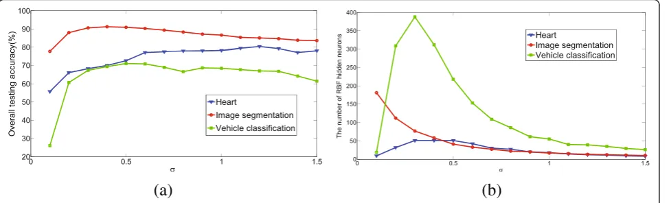
Figure 11a, b shows the impact of width on the overall classification accuracy and the number of RBF hidden neurons, respectively. Figure 11 illustrates that for the Heart and VC data sets, when the width parameter is small, such as σ= 0.1 and σ= 0.2, the overall classifica-tion accuracy is poor, and effective coverage of the input sample space is not achieved.
When the value of the width parameter is in a suitable range, the number of generated RBF hidden neurons will change, but a relatively stable classification accuracy can be achieved. For the proposed ILRBF-BP algorithm, once the width is given, it can learn the sample space auto-matically, and the changes in the width parameter will affect the coverage of RBF hidden neurons and generate different RBF hidden neurons. Thus, the incremental learning strategy can counteract the effect of the width to some extent.
4 Impact of the number of BP hidden neurons on ILRBF-BP
In the hybrid RBF-BP network architecture, the nonlin-ear BP algorithm is used to adjust the weights of the MLPs, which further improves the classification result. However, this method results in an increase in the num-ber of parameters to be selected, especially the selection of the number of BP hidden neurons. For this problem, we conduct experiments on the UCI data sets and dis-cuss the results.
(a)
(b)
Figure 12 shows the impact of the number of BP hid-den neurons on ILRBF-BP. For the Heart, IS, and VC problems, when the number of BP hidden neurons is greater or equal to 4, the overall classification accuracy does not change considerably. For the hybrid RBF-BP network, the mapping results of RBF hidden neurons are processed and used for the input of BP network, which improves the stability of the BP network and effectively avoids falling into local minima for the BP algorithm. Thus, the dependence on the number of BP hidden neu-rons is reduced. When the sample set is more complex, the momentum term can be used to improve the BP algorithm further.
5 Conclusions
In this paper, an incremental learning algorithm for the hybrid RBP-BP (ILRBF-BP) network classifier is proposed. The ILRBF-BP algorithm uses a potential function to measure the density of the training sam-ple space and incrementally generates RBF hidden neurons, enabling the effective estimation of the cen-ter and number of RBF hidden neurons. In this way, a suitable network size for RBF hidden layer that matches the complexity of the sample space can be built up. A hybrid RBF-BP network architecture is designed to improve classification performance fur-ther, which shows good stability and generalization performance. The hybrid network simplifies the selec-tion of the number of neurons in the BP hidden layer while further reducing the dependence on space map-ping in the RBF hidden layer.
The performance of the ILRBF-BP algorithm has been compared with other batch learning algorithms, such as SGBP, KM-RBF, SVM, and ELM, and sequential learning algorithms, such as MRAN, GAP-RBF, and OS-ELM, in artificial data sets and UCI data sets. The method of adjusting output label values is used to prevent the
output saturation problem for multi-class classification. Experiments demonstrate the superiority of the ILRBF-BP algorithm.
In the future, we will focus on the optimization of kernel width and imbalanced data classification prob-lems. In the ILRBF-BP algorithm, the width is fixed and selected by cross validation and the adjustment of width parameter will affect the location of next center, as well as the network size. Therefore, it is necessary to design an adaptive width adjustment to adapt to the different regions of the sample space. In addition, for the imbal-anced data classification problem, the samples in the boundary regions contain more classification informa-tion, thus how to measure and select these samples is particularly important. Further studies are needed to address these concerns.
Competing interests
The authors declare that they have no competing interests.
Acknowledgements
The authors thank the support provided by the National Science Foundation of China (No. 61331021, U1301251) and the Shenzhen Science and Technology Plan Project (JCYJ20130408173025036). The authors would like to thank the Editor-in-Chief, the Associate Editor, and the Anonymous Reviewers for their helpful comments and suggestions which have greatly improved the quality of presentation.
Received: 3 November 2015 Accepted: 27 April 2016
References
1. M Lin, K Tang, X Yao, Dynamic sampling approach to training neural networks for multiclass imbalance classification. IEEE Trans Neural Netw and Learning Systems24(4), 647–660 (2013)
2. L-Q Li, W-X Xie, Intuitionistic fuzzy joint probabilistic data association filter and its application to multitarget tracking. Signal Process96, 433–444 (2014) 3. Y-L Wei, J-B Qiu, HR Karimi, M Wang, H-infinity model reduction for
continuous-time Markovian jump systems with incomplete statistics of mode information. Int J Syst Sci45(7), 1496–1507 (2014)
4. Y-L Wei, J-B Qiu, HR Karimi, M Wang, Filtering design for two-dimensional Markovian jump systems with state-delays and deficient mode information. Inform Sci269, 316–331 (2014)
5. Y-L Wei, J-B Qiu, HR Karimi, M Wang, A new design of H∞filtering for continuous-time Markovian jump systems with time-varying delay and partially accessible mode information. Signal Process93(9), 2392–2407 (2013) 6. F-Y Meng, X Li, J-H Pei, A feature point matching based on spatial order
constraints bilateral-neighbor vote. IEEE Trans Image Process24(11), 4160–4171 (2015)
7. L-X Guan, W-X Xie, J-H Pei, Segmented minimum noise fraction transformation for efficient feature extraction of hyperspectral images. Pattern Recogn48(10), 3216–3226 (2015)
8. HC Nejad, O Khayat, B Azadbakht, M Mohammadi, Using feed forward neural network for electrocardiogram signal analysis in chaotic domain. J Intelligent and Fuzzy Systems27(5), 2289–2296 (2014)
9. CH Weng, CK Huang, RP Han, Disease prediction with different types of neural network classifiers. Telematics Inform33(2), 277–292 (2016) 10. C Lu, N Ma, ZP Wang, Fault detection for hydraulic pump based on chaotic
parallel RBF network. EURASIP J on Advances in Signal Processing49, (2011). doi: 10.1186/1687-6180-2011-49
11. J Moody, CJ Darken, Fast learning in networks of locally-tuned processing. Neurocomputing1(2), 281–294 (1989)
12. D Lowe, Characterising complexity by the degrees of freedom in a radial basis function network. Neurocomputing19(1-3), 199–209 (1998) 13. J Platt, A resource-allocating network for function interpolation. Neural
Comput3(2), 213–225 (1991)
14. V Kadirkamanathan, M Niranjan, A function estimation approach to sequential learning with neural networks. Neural Comput5(6), 954–975 (1993) 15. L Yingwei, N Sundararajan, P Saratchandran, A sequential learning scheme
for function approximation using minimal radial basis function. Neural Comput9(2), 461–478 (1997)
16. G-B Huang, P Saratchandran, N Sundararajan, An efficient sequential learning algorithm for growing and pruning RBF (GAP-RBF) networks. IEEE Trans Syst Man Cybern B Cybern34(6), 2284–2292 (2004)
17. G-B Huang, P Saratchandran, N Sundararajan, A generalized growing and pruning RBF (GAP-RBF) neural network for function approximation. IEEE Trans Neural Netw16(1), 57–67 (2005)
18. M Bortman, M Aladjem, A growing and pruning method for radial basis function networks. IEEE Trans Neural Netw20(6), 1030–1045 (2009) 19. H Yu, PD Reiner, T Xie, T Bartczak, BM Wilamowski, An incremental design
of radial basis function networks. IEEE Trans Neural Netw and Learning Systems2(10), 1793–1803 (2014)
20. S Suresh, D Keming, HJ Kim, A sequential learning algorithm for self-adaptive resource allocation network classifier. Neurocomputing73(16-18), 3012–3019 (2010)
21. T Xie, H Yu, J Hewlett, P Rózycki, B Wilamowski, Fast and efficient second-order method for training radial basis function networks. IEEE Trans Neural Netw and Learning Systems23(4), 609–619 (2012)
22. C Constantinopoulos, A Likas, An incremental training method for the probabilistic RBF network. IEEE Trans Neural Netw17(4), 966–974 (2006) 23. G-B Huang, Q-Y Zhu, C-K Siew, A new learning scheme of feedforward
neural, inProceedings of International Joint Conference on Neural Networks (IJCNN 2004), pp. 985–99
24. N-Y Liang, G-B Huang, P Saratchandran, N Sundararajan, A fast and accurate online sequential learning algorithm for feedforward networks. IEEE Trans Neural Netw17(6), 1411–1423 (2006)
25. G-B Huang, L CHEN, C-K Siew, Universal approximation using incremental constructive feedforward networks with random hidden nodes. IEEE Trans Neural Netw17(4), 879–892 (2006)
26. G-B Huang, L CHEN, Convex incremental extreme learning machine. Neurocomputing70(16-18), 3056–3062 (2007)
27. G-B Huang, L Chen, Enhanced random search based incremental extreme learning machine. Neurocomputing71(16-18), 3460–3468 (2008) 28. G Feng, G-B Huang, Q Lin, Error minimized extreme learning machine with
growth of hidden nodes and incremental learning. IEEE Trans Neural Netw 20(8), 1352–1357 (2009)
29. Y LeCun, L Bottou, GB Orr, K-R Müller, Efficient backprop. Lecture Notes Comput Sci1524, 9–50 (1998)
30. J-H Pei, W-X Xie, Adaptive multi thresholds image segmentation based on potential function clustering. Chinese J Computers22(7), 758–762 (1999) 31. OA Bashkerov, EM Braverman, IB Muchnik, Potential function algorithms
for pattern recognition learning machines. Autom Remote Control25(5), 692–695 (1964)
32. G Cybenko, Approximation by superpositions of a sigmoidal function. Mathematics of Control, Signal, and Systems2, 303–314 (1989) 33. S Hayin,Neural networks and learning machines. Third Edition(China
Machine Press, China, 2009), pp. 61–63
34. C Blake, C Merz,UCI repository of machine learning databases(Department of Information and Computer Sciences, University of California, Irvine, 1998). available at http://archive.ics.uci.edu/ml/
35. C-C Chang, C-J,LIBSVM: a library for support vector machines(Department of Computer Science and Information Engineering, National Taiwan University, Taiwan, 2003). available at http://www.csie.ntu.edu.tw/~cjlin/libsvm/index. html
Submit your manuscript to a
journal and benefi t from:
7Convenient online submission
7Rigorous peer review
7Immediate publication on acceptance
7Open access: articles freely available online 7High visibility within the fi eld
7Retaining the copyright to your article