Centre for Advanced Spatial Analysis University College London
1-19 Torrington Place Gower Street
London WC1E 6BT Tel: +44 (0) 171 391 1782 Fax: +44 (0) 171 813 2843 Email: [email protected] http://www.casa.ucl.ac.uk/
http://www.casa.ucl.ac.uk/multi_agent.pdf
Date: April 1999 ISSN: 1467-1298
ABSTRACT
As part of the long term quest to develop more disaggregate, temporally dynamic models of spatial behaviour, micro-simulation has evolved to the point where the actions of many individuals can be computed. These multi-agent systems/simulation (MAS) models are a consequence of much better micro data, more powerful and user-friendly computer environments often based on parallel processing, and the generally recognised need in spatial science for modelling temporal process. In this paper, we develop a series of multi-agent models which operate in cellular space. These demonstrate the well-known principle that local action can give rise to global pattern but also how such pattern emerges as the consequence of positive feedback and learned behaviour. We first summarise the way cellular representation is important in adding new process functionality to GIS, and the way this is effected through ideas from cellular automata (CA) modelling. We then outline the key ideas of multi-agent simulation and this sets the scene for three applications to problems involving the use of agents to explore geographic space. We first illustrate how agents can be programmed to search route networks, finding shortest routes in ad hoc as well as structured ways equivalent to the operation of the Bellman-Dijkstra algorithm. We then demonstrate how the agent-based approach can be used to simulate the dynamics of water flow, implying that such models can be used to effectively model the evolution of river systems. Finally we show how agents can detect the geometric properties of space, generating powerful results that are not possible using conventional geometry, and we illustrate these ideas by computing the visual fields or isovists associated with different viewpoints within the Tate Gallery. Our forays into MAS are all based on developing reactive agent models with minimal interaction and we conclude with suggestions for how these models might incorporate cognition, planning, and stronger positive feedbacks between agents.
ACKNOWLEDGEMENTS
Introduction
Space-time dynamics is receiving increased attention in GIS as the need to make such technologies
sensitive and relevant to both traditional and state-of-the-art geographic theory is recognised.
Various starting points for these developments have emerged. In mainstream GIS, temporal data
models have been proposed and examined (Clifford and Tuzhilin, 1995; Egenhofer and Golledge,
1998; and Langran, 1992) but more directed research has come from theory and model development
outside the field, for example in the development of models based on nonlinear dynamics with no
strict spatial framework and in discrete versions of these models such as those based on cellular
automata (CA). This variety of modelling, however, does not yet have the kind of database support
which temporal GIS provides although there are strong links to raster-based GIS.
In contrast, object-based GIS provides the potential for simulating individual actions and decisions
in space. Recently, the idea of agents has become popular as computer systems themselves have
become highly decentralised and as it has become increasingly necessary to evolve software objects
that can keep track of complex network systems. In fact, such multi-agent systems/simulations
(MAS) are now providing alternative approaches to modelling space-time dynamics in a variety of
disciplines where computing is essential to applications. Such approaches initially developed from
ideas in from distributed artificial intelligence where the key idea is that programmed behaviour
depends entirely on algorithms based on artificial worlds or environments inhabited by interacting
processes. Such systems are able to simulate complexity through the interaction of individuals or
agents comprising large populations where each agent would act and interact locally. These
multi-agent simulations are thus quite suggestive for space-time dynamics in that they allow exploration
of relationships between micro-level individual actions and emergent macro-level phenomena. This
in turn links their operation to CA models where global dynamics and spatial pattern is a
consequence of local action.
In this paper, we will explore these relationships, beginning with a summary of cell-based
modelling in GIS and the way CA models are beginning to inform spatial simulation. We then
move to describe, albeit very briefly, the ideas behind agent-based modelling and multi-agent
simulations. We then demonstrate that CA and agent-based models provide a firm base for
space-time dynamics and illustrate these notions with three applications: route finding in systems where
distance and direction are largely unknown but need to be explored by agents rather than computed
geometrically; spatial systems where gradients are important in directing movement and location
such as river systems and watersheds; and systems where viewsheds are critical to measuring
geometric properties such as in building complexes and landscapes. Our emphasis here will thus be
is the modus operandi, and where our focus in on the exploration of space-time rather than on the
simulation of human behaviour per se.
Cell-Based GIS and Cellular Automata (CA) Modelling
Cell-based GIS originates from data systems where the unit of representation is identical and
regularly distributed such as those based on pixels, grids or any other regular tessellation of the
plane. Typically spatial representation in such systems is based on a hierarchy of levels deriving
from the cell at its most local level which is the basic unit of operation. Neighbourhoods are thence
defined around each cell, usually formed from the cells at the 8 compass directions (where the cells
are arranged in a grid), and this links such models formally to cellular automata where
neighbourhoods are the basic structures within which action and decision take place. A higher level
in which neighbourhoods (and of course the cells that comprise them) are arranged into zones is
often defined as the focal level and this is akin to idea of the field which also appears in some CA
models (Xie, 1996). Finally the top level is global where actions take place across the entire system.
Sometimes this level is referred to as the world or the environment. A useful summary of these
concepts is given by Gao et al. (1993).
Cell-based operations in such systems are based on the conventional idea of layers which are
combined in various ways. Map algebra is the most obvious way of transforming layers through
local operators whose functions embody the normal arithmetical and statistical functions often
arranged in subtle ways to enable recoding and classification. Operations can be employed at any
level but vary in that as the system is aggregated from cells into neighbourhoods into zones and
thence into its entire world, the types of operations change, distance measures becoming
increasingly important. At the highest levels, weighting and normalisation are essential functions.
Although map algebra provides a valuable set of procedures, it inherently lacks the ability to deal
with the temporal dimension, nor as Takeyama and Couclelis (1997) in particular stress, does it deal
explicitly with spatial relations and interaction among locations. In contrast, cellular automata
modelling is essentially designed to simulate the dynamics of spatial interaction, although the
emphasis is entirely local. With map algebra, it shares a number of concepts such as the world,
neighbourhood, and cell but because of its focus on change and decision through time, CA
embodies three dynamic elements: the idea of the system state, the notion of transition and rules for
CA models have been quite widely applied in geographical modelling although to date their
development has not been very intensive. Models based on urban and regional dynamics are
significant (see White 1998 for a review) but the main problems have been twofold: developing
spatial interaction in spaces wider than the neighbourhood itself and in enabling the model
dynamics to take account of system-wide conservation constraints which are usually destroyed by
CA transitions in that growth and change are driven from the bottom up. A number of
environmental models based on CA where local action is perhaps more significant than in urban
systems, have been developed. The most promising areas involve wildfire propagation (Clarke and
Olsen 1993), and ecosystem functioning based on predator-prey relationships (Camara et al. 1996).
Burrough (1998) has recently suggested that temporal dynamics within GIS might be based on a
tool kit comprised of the key elements of CA and cell-based GIS representations including map
algebra.
Fully integrated systems incorporating GIS, CA, and map algebra have also been considered.
Wagner (1997) has examined the similarities between CA and raster GIS where he illustrates the
potential of implementing one within the another while Takeyama and Couclelis (1997) go further
in proposing a general mathematical framework for the integration of GIS and CA based on the
notion of proximal space. However the basic problem with such models is that the concept of space
is quite restrictive. Thinking of the elements of a geographical system as simply cells poses many
difficulties especially as it is difficult to ascribe more than one set of transition rules to each cell and
different mixes of states to the same cell. Such extensions can be implemented but only by
disaggregating cells to more basic units, that is, to ever finer cells. To make progress without losing
the intrinsic benefits of local operations across cells, what is required is a more active set of objects
associated with those cells. Multi-agent simulations are being developed to meet this challenge.
MAS: Multi-Agent Systems and Simulations
We must first discuss the generic idea of an agent for this is basic to the models that we are working
with. Essentially agents are autonomous entities or objects which act independently of one another,
although they may act in concert, depending upon various conditions which are displayed by other
agents or the system in which they exist. Franklin and Graesser (1997) formalise the definition of an
autonomous agent as “a system situated within and a part of an environment that senses that
environment and acts on it, over time, in pursuit of its own agenda and so as to effect what it senses
in the future”. Autonomous agents thus cover a wide variety of behaving objects from humans and
other animals or plants to mobile robots, creatures from artificial life, and software agents. The key
quite different regimes. In this sense, the concept of an agent is as wide as that of the object in
software engineering.
Firstly, agents operate within environments to which they are uniquely adapted and just as there
may be more than one type of agent in a simulation, there may be more than one kind of
environment. In this context, the kinds of environments that we will deal with are by their nature
‘distributed’. Spatial systems are extensive and in the form of cellular space, have the potential to
represent highly decentralised behaviour. Indeed this is an intrinsic property of CA modelling. In
fact there is an entire range of different kinds of environment from distributed to highly centralised
(Ferber 1999) and it is not out of the question that MAS in a GIS context might even be fashioned
in more centralised terms. Much will depend upon the area of application and the elements of the
system to be modelled.
Secondly, the ways in which agents ‘sense’ and ‘act’ in their environment are central determinants
of the behaviour which is to be modelled. Agents can be classified in many ways: a key distinction
is between ‘reactive’ agents and ‘cognitive’ (or deliberative) agents, the difference being with
respect to the conditions which drive the ‘senses’ and ‘actions’ of the agent. For example, a reactive
agent is just as autonomous as a cognitive one but the central difference is that the reactive agent
will behave entirely by reacting to its environment or to other agents. A cognitive agent may do the
same but will also behave according to its own protocols or plans which in turn embody the idea
that agents have goals that are unique to themselves and which drive their behaviour.
To describe an autonomous agent, it is necessary to describe its environment, sensing capabilities,
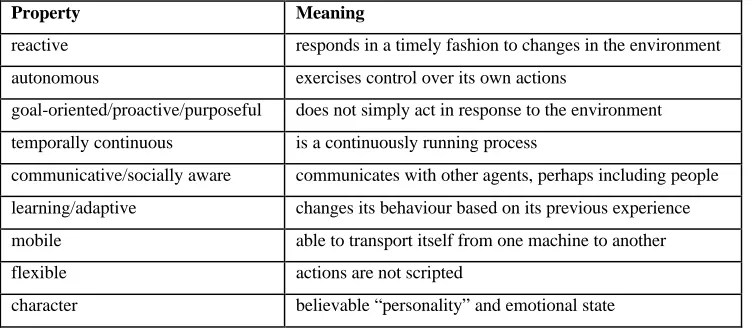
and actions. Franklin and Graesser (1997) have proposed a range of properties which we present in
Table 1.
Property Meaning
reactive responds in a timely fashion to changes in the environment
autonomous exercises control over its own actions
goal-oriented/proactive/purposeful does not simply act in response to the environment
temporally continuous is a continuously running process
communicative/socially aware communicates with other agents, perhaps including people
learning/adaptive changes its behaviour based on its previous experience
mobile able to transport itself from one machine to another
flexible actions are not scripted
character believable “personality” and emotional state
These range from the most ‘passive’ agents which are essentially reactive, to agents that display the
kind of intelligence and foresight that we associate with ourselves, with our own cognition.
However a central feature of whatever class of agent we are dealing with is their ability to
communicate which enables them to interact, directly or indirectly with one another as well as sense
and respond to their environment. Interaction between agents can thus take place through the
environment which acts as the intermediary.
This kind of agent technology is being slowly developed with geographic systems in mind.
Rodrigues et al. (1996) employ spatial agents for geographic information processing. They have
defined spatial agents as agents that make concepts computable for purposes of spatial simulation,
spatial decision making, and interface design. But agent-based simulation is perhaps most
appropriate where local spatial operations are the focus and this suggests that physical, human, and
software systems where spatial movement and location is primarily structured in terms of
neighbourhood action are the best candidates for application. In this sense, we can consider putting
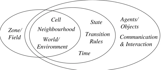
MAS together with cell-based and CA models. We illustrate the correspondence of these ideas in
Figure 1 which shows that as we move from cell-based to CA through to MAS, then our systems
become ever more active in the temporally dynamic sense and ever more decentralised in terms of
spatial decision-making. The models we will present below have all the characteristics of the set of
concepts illustrated here.
There are now some significant applications of multi-agent models which are beginning to define
the field, many of which are designed around appropriate software. Unlike the earlier generation of
models in geography, software is increas-ingly beginning to guide their formulation and in fact, the
very existence of agent-based models depends upon the development of object-oriented software.
Considerable effort has been made in order to provide a easily used software platform for scientists
to undertake studies on complex systems. The SWARM project (Langton et al. 1995) is one of the
most ambitious in that it is designed to serve as a generic platform for modelling and simulating
complex behaviour in which agents are akin to those of artificial life. It provides a set of classes for
defining agent behaviour using the computer language ‘Objective C’. Based on this system, various
spatial projects are being developed such as the micro-simulation traffic model - TRANSIMS as
well as our own pedestrian model of Wolverhampton STREETS (Schelhorn et al., 1999). SWARM is
not as easy to implement as might appear although attempts are being made to provide more
user-friendly versions (Gulyás et al. 1999). Less general but nevertheless quite highly structured
dynamic models are being built with specific software: for example, Epstein and Axtell’s (1996)
Sugarscape model which attempts to simulate the evolution of an artificial society and Batty, Xie
Zone/
Field World/ Environment
Cell Neighbourhood
State Transition Rules
Agents/ Objects Communication & Interaction Time
Figure 1: Relations Between Cell-Based GIS, CA Modelling, and MAS
The software we use here is based on a massively parallel implementation of the graphics language
Logo. StarLogo as it is called by its originator (Resnick, 1994), is a language for CA modelling but
with agents forming the critical action elements of the system. In effect, agents are able to roam
across the space and sense the environment which is composed of cells. The key operations within
the software enable agents to react to what is within their neighbourhood which in turn is based on
information which is encoded within the cells forming their environment. Of course, agents can
react to one another but in general, action at a distance is difficult although not impossible to
represent within the software. The software has evolved to a point where realistic applications can
now be made although it is still largely focused on instructional use. Various applications have been
developed for simulating real-life phenomena such as bird flocks, traffic jams, ant colonies, and
market economies. A useful set of extendible models is available at
http://www.ccl.tufts.edu/cm/models/.
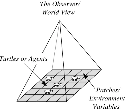
StarLogo consists of three elements: turtles which are agents, patches which constitute the cells of
the environment, and the world view which is called the observer. Turtles are autonomous agents
existing in CA-like space, each cell of which is a patch. Interactions can occur between turtles,
between turtles and patches, and between the observer and each of these elements. These
interactions are largely visual, economic, or chemical in terms of the functions that enable them.
Agents move according to their angular heading but various distance operators are available. There
is no central coordination in the software for the observer simply acts to pass global information
down to patches and agents and to organise the software displays. A picture of how the framework
Turtles or Agents
Patches/ Environment Variables The Observer/
World View
Figure 2: The Turtle-Patch-Observer Structure of StarLogo
Finally, there is an impressive range of output functions for the software which make its
demonstration effective and appealing. The interface, in fact, is shown in the next two figures below
although in this paper, we will not dwell any further on the software, for this is simply a means to
the end.
Movement in Cellular Space: Navigating by the Stars and the Sun
To develop multi-agent models that operate in cellular space, we must first introduce some formal
notation. We will define each agent, or walker in our first example, by an identity k for a set of K
agents (where k = 1, 2, …, K) and a time t which is associated with when the agent acts in making some spatial decision involving movement, location, or interaction. w tk( ) is thus the state of the
agent which for our purposes can remain implicit although might constitute whether the agent is at
rest or in motion or has some attribute associated with their spatial decision-making. Agents locate
or move in cellular space which is defined according to the conventions of cellular automata
modelling. Agents for example act locally in their immediate neighbourhood defined as the 8
adjacent cells (the Moore neighbourhood) surrounding their current location which is in turn given
by the grid coordinates (x, y). We will use x and y to define distances within the grid but for
purposes of reference we will also refer to coordinates x and y by their row and column identifiers i
and j as xi and yj. The state of a typical walker is now given as wk( ,x y ti j, ) which can also be written as wkij( ) .t
Motion in these models is always controlled by the angular heading θk( ) which is associated witht
move one cell step in its surrounding neighbourhood. Given a heading θk( ) , an agent will walk tot
a new location with coordinates x ti( +1),y tj( +1)
x ti( + =1) x ti( )+∆x and y tj( + =1) y tj( )+∆y (1) ∆x=rcosθk( )t and ∆y=rsinθk( )t . (2)
As the step distance r is always assumed to be 1 which implies that agents always walk at the same
speed, then equations (1) can be rewritten as
x ti( + =1) x ti( )+cosθk( )t and
y tj( + =1) y tj( )+sinθk( )t . (3)
Motion is only possible within the Moore neighbourhood, and thus the heading θk( ) ist
approximated to one of the eight points of the compass around x ti( ) and y tj( ) , this set being
{ 0 1 4,( ) , (π 1 2) , (π 3 4) , , (π π 5 4) , (π 3 2) ,π and (7 4)π }.
In many of our applications, movement or location takes place in space which is less than the dimensions of the entire cellular system. We show this by defining a constraints variable C x y( ,i j) as the state of the cellular system at each location x yi, j where
C xi y j
x ,yi j
( , )
,
=
0 1
otherwise if movement or location in is permitted
. (4)
In our first example in this section, C x y( ,i j) will define a street or path system, with predominantly linear features which marks out the permissible routes along which movement might take place. In
other applications, this variable can be used to impose any kind of areal constraint on the system
such as areas which cannot be visited or developed due to physical or institutional limitations.
We now need to illustrate how movement and other actions based on equation (3) is affected by the constraints in equation (4). For this, we can prime the location coordinates as x ti' y t'j
( +1), ( +1 to)
indicate that these are ‘predicted’ rather than actual locations. To check if movement to these
predicted locations is feasible, we must make the following test:
if C x y( ,i j)=1 , then x ti x ti
'
( + =1) ( +1 and ) y tj y tj
'
( + =1) ( +1)
obstacle-There are many possibilities for avoiding obstacles but all these involve testing different, alternative
directions to see what is possible. The simplest of these is to choose a feasible direction where
C x y( ,i j)=1 for any of the remaining 7 compass points which have not been evaluated so far. It,
may be necessary to repeat the procedure until such a feasible direction is discovered although this
will always be possible in the systems that we are dealing with here. The basis of this algorithm is
as follows:
if C x y( ,i' 'j)=0 , then θk'( )t =random (π)
x ti'( + =1) x ti( )+cosθk'( )t , and
y t'j( + =1) y tj( )+sinθk'( )t
until C x y( ,i j) ,
' ' =
1 . (5)
This is the simplest algorithm which enables agents to walk around obstacles but it destroys the
original heading, in that it substitutes this for random direction. If many walkers are launched from
a single point in the system and given random headings to begin with, then in a system of connected
streets, the steady state distribution of agents will mirror the density of the street pattern in that
walkers will be distributed evenly (in statistical terms) per unit of street. Of course the configuration
of the streets is important in this because the density of streets themselves per unit of area may well
vary but nevertheless, this algorithm and the method of walking leads to uniformity in the probabilistic sense. If the heading θk( ) which is initially established is critical, then the algorithmt
in (5) above can be easily altered to reflect successive small changes ε to θk'( ) which ultimatelyt
lead to a direction which is as near as possible to the original one but is then feasible. Feedback can
be built into the algorithm as other agents can be regarded as obstacles to avoid although we have
not implemented this kind of interaction in the obstacle-avoidance procedures used here.
Our thesis here is that multi-agent systems are useful not only for simulating spatial systems at the
micro level but for actually exploring the properties of space that may not be accessible in any other
way. Agents may well explore space as part of their behaviour but in this context we are focusing
primarily on the use of agents to sense properties of systems that could not be measured or detected
in any other way. Our first problem is one in which many walkers in the system need to find routes
to different places which act as their destinations. The problem is to find ‘feasible’ but not
necessarily shortest routes for these walkers from any and every point in the system to these
destinations. The walkers know where their destinations are in global terms - in terms of their
coordinates - but do not know how to get to those coordinates and thus need to explore the local street systems purposefully en route to these destinations. For each walker k, wk( ,x y ti j, ) , we can
route system and must thus make their way to the destination from their global knowledge of
Xk,Yk and from their ability to explore the street system locally avoiding obstacles, as we have already shown. Then from any location x yi, j, the shortest distance to the destination as the crow
flies for any agent k is
[
]
r x yk( ,i j)= (xi −Xk) +(yji −Yk)
−
2 2
1
2 (6)
where the heading can be computed as
θk i j
i k k i j
x y x X
r x y
( , ) cos ( )
( , ) = − −1 . (7)
The model works as follows. Given any distribution of walkers {wk( ,x y ti j, ) }, each walker fixes
their heading from equations (6) and (7), and makes a first step which is checked using the
obstacle-avoidance routine in equation (5). Because the heading is important, then walkers do not want to
deviate from this heading too much. If they need to modify their heading to avoid an obstacles, they gradually modify their heading as θk x yi j θk x yi j δk
" '
( , )= ( , )+ where δk is a very small increment to the angle. This is used in the algorithm in (5) and ensures that the correction to the global heading
will be as small as possible. In essence, this model assumes that walkers navigate from their
‘knowledge of the stars and the sun’: they know the location of their destinations - the stars or sun at Xk,Yk - but have to creep around the street system, mainly hugging the walls of the streets until
they eventually reach their destinations. Much depends upon the local configuration because they
might get stuck. It may be necessary to go further away from the destination at some point to
actually get to it and thus the only way to do this is to give walkers some greater perturbation in
their heading, letting them walk “the wrong way” for some little time. In fact, the original algorithm
with random headings will ensure that most local loops are avoided. We have programmed several
variants of the obstacle-avoidance algorithm for an hypothetical street system and we show a
realisation of the path traced for one walker to one destination in Figure 3. Note how the path
Figure 3: Approximating Shortest Routes by Global Navigation and Local Search
More Purposive Navigation: Shortest Routes
The best developed navigation problem enables an exact calculation of the shortest routes between
any origin and destination on a route system which is strongly connected in the graph-theoretic
sense. We will digress a little and sketch the classic problem before we reformulate this in
agent-based terms. We will call origins m and destinations n, and we will code the route network using the constraint variable C x y( ,i j) where the distance dmn between any origin m and destination n is now
computed as
[
]
dmn = xim −xin + yjm −yjn
−
( )2 ( )2
1
2 . (8)
Note that m n, ∈N where N is the set of nodes and each node is associated with the coordinate pairs
defined in equation (8). This problem is well-known and soluble using the Bellman-Dijkstra
algorithm which was discovered 40 years ago. Starting from any origin node O, it is possible to
compute all the shortest paths to the other N-1 nodes from
{
}
ft n f d
m t m mn
+1, =min , + (9)
where ft+1,n is the minimum distance so far at the t+1thstep of the algorithm. The procedure begins with f1,n =dOn, and essentially involves systematically tracing through all the routes of the
The usual problem is one where we know the nodes or junctions between the routes in the network
and we know the distances between these nodes. However imagine a system in which we do not
‘yet’ know the location of the streets or the junctions and thus we have no idea how far it is between
these unknown nodes. Thus the problem involves finding the junctions and the distances between
the routes before the shortest routes can be found. However with the walker behaviour defined in
the previous section, we can explore the space so that we can decide whether or not a cell in
C x y( ,i j) is a node. We know that if the cell C x y( ,i j) =1, then it is part of a route and we can then
define a junction as a cell which has more than 2 positive cells in the eight cells that constitute its
Moore neighbourhood. At every stage of the walk, we can thus decide if the cell is a node. As we
walk between nodes (because we will always assume the origin O is a node from which all walking
begins), then we can also count the distance travelled and in this way build up knowledge of local
distances within the system. This kind of problem is not unusual where data is provided in raster
form from satellite or where the system is so complex, that no graph theoretic definition of nodes
and route distances has been made beforehand.
We can get a sense of how the model works from the following algorithm
Start at the Origin O which is a node
Find out how many exits there are from the node (s)
Find out how many routes from these exits have already been traversed
Generate as many new agents as there are routes to be traversed, each having memory of the minimum distance to that node so far
Set the heading of the relevant agent along its route
Walk one step of the route at a time, count the distance travelled
Check for the existence of a node
If a node is encountered STOP; if not go back to
Check all agents entering node; choose the agent with the minimum distance so far, as the minimum distance for the node
Check if all nodes have been visited and all routes traversed If YES, STOP; if NO then go back to
↓ ⊗
↓
↓
↓
↓ ⊗ ⊗
↓
↓
⊗ ⊗ ↓
↓
⊗
Although the algorithm starts at node O, eventually the full set of nodes are encountered. A full
We can explain how the algorithm works more effectively by tracing through an example. Imagine
that we start at an origin node where there are three exit routes. We create three agents, give them a
memory of zero distance, and then send them off along their respective routes, checking for the
existence of junctions, and counting the increment of distance travelled one step at a time. When
they encounter a node they stop, and we wait until all three have reached this state, before we check
the status of the problem. On this first pass through, we know that there are more routes to traverse
from the three new nodes at the end of the three routes encountered (unless we have a triangular set
of routes), so we take the shortest distances computed on these first three routes and find out how
many new routes there are from the three nodes encountered. We dissolve the existing agents and
from each of the three nodes, create as many agents as we need at each node so they can traverse
the next set of routes. We give these agents memory of the shortest distance to date and off they go
following the same procedure as previously. When they have all encountered nodes, we check to
see if the routes from these new nodes have been traversed. If not we create new agents, and choose
the shortest distance of any of the agents entering the nodes as the new memories of distance for the
new agents. Note that at this point, we may have two or more agents entering a node from different
routes (which will be the usual condition for networks with more than about 10 nodes), and thus we
need to take the minimum distance associated with one of these agents. Eventually we will run out
of nodes to visit and routes to traverse and at this point the minimum distances associated with the
any of the agents at each node are the shortest routes from the origin to each of these nodes.
It is worth noting that at each step, we need to find out whether the pixel that the agent is on is a
junction or not. We are also assuming that the route has been marked out by a single line of pixels, not by the full width of the street as shown in the examples. Then at each location x yi, j
if C x yi j i i i
j j j
( , )> ,
− < < + − < < +
∑
31 1
1 1
then x yi, j is a junction . (10)
We also need to compute the directions of the exits from the junction, check to see if the routes
from these exits have been traversed, and give the agents who are created to leave the junction from
these exits, the shortest distance to this junction computed so far. Note that agents communicate
with one another when they have entered as node in that they pass their knowledge of distance
travelled so far to the new agents who choose the minimum. It is also possible that in some systems
depending upon how the pixels are configured to represent the routes, that the algorithm in equation
(5) might be necessary to keep the walker on track along the route in question.
out which is equivalent to that used in the global navigation model in Figure 3. In this latter case,
we have to store the nodes forming the shortest path as we discover these, and in the software we
are using this is both cumbersome and expensive in terms of memory. Nevertheless, this example
shows how effective agent-based models can be in exploring systems whose properties are largely
unknown the analyst prior to exploration. The next example takes this one stage further.
Figure 4: Agent-Based Implementation of the Bellman-Dijkstra Algorithm
Watershed Dynamics: The Evolution of River Systems
We have seen how agent-based models can be used to track spatial properties associated with route
and network systems which are highly constrained but equally effective procedures exist for cellular
systems composed of surfaces. Indeed, the original application of cellular systems in GIS for
overlay analysis and map algebra in landscape planning are largely based around operations on
surfaces. In this example, we associate agents with particles of moisture - rain droplets - falling on a
landscape or indeed any phenomena which affects a surface such as pollution particles. In essence,
when particles fall on a surface, they move across the surface; the usual assumption is that they
move according to the principle of least effort, in the direction of the steepest gradients. Our model
here simply traces the paths of these particles demonstrating how local action/movement creates
patterns that have a global morphology.
We first generate or observe a set of particles or agentswk(x yi, j, )1 at different locationsx yi, j at initial time t=1. These agents might be randomly generated and as such act as sources for motion
‘walking’ locally one step at a time according to the logic in equations (1) to (3). But in this case,
the heading is not computed randomly or globally but in terms of the local gradient of the surface
S x y( i, j) . The standard approximation to this gradient is given as
grad ( ,x y ) x S x y( , ) ( , )
x y
S x y
y i j i j i i j j ≈∆ ∂ +∆ ∂ ∂
∂ , (11)
but in terms of the model implementation which is constrained to the Moore neighbourhood, then
the minimum gradient and its appropriate direction is computed from
{
}
min grad { , }
, ,
( , ) { ( ) ( )}
{( ) ( ) }
i j i j
i j i j
i i j j
x y S x y S x y
x x y y
± ± ± ±
± ±
± ± −
= −
− + −
1 1 1 1
1 1
1 2
1
2 1 2 . (12)
From the direction, we need to compute the appropriate heading, and then movement occurs
according to the motion implied by equations (1) to (3).
From the initial configuration of agents {wk(x yi, j, )1 }, we trace out the paths formed by movement
across the surface. These paths follow the steepest local gradients and essentially can be interpreted
as continuing sources of water - springs if you like - which produce rivers across the surface. Of
course this is not the way rivers are formed but simply give river-like patterns. However as the
distribution across the surface is random and takes no account of the fact that rivers are usually
sourced on higher terrain, then the patterns produced are unrealistic. Moreover, when there is no
exit from the landscape in terms of the terrain, lakes should form and the sinks shown in the
examples below indicate where these lakes would be. Strictly speaking we could modify the
program to account for this but there are many other features we need to develop first. Insofar as
agents communicate with each other in this model they do so when they join each other in a stream
or lake.
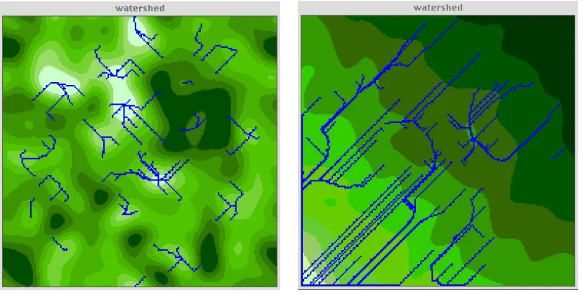
In Figures 5(a) and 5(b), we show two examples of these simulations of watershed dynamics in
terms of the terrain traces across two different landscapes. The first landscape in Figure 5(a)
contains sources and sinks but no general drainage out of the region. In Figure 5(b), we show an
example of the pattern which is more dendrite in form which emerges when the general gradient of
the terrain falls from north-east to south-west. What these examples both demonstrate is the classic
conclusion that local action gives rise to global pattern, in this case fractal patterns which result
from the action of movement which in essence is space-filling. However the terrain is somewhat
artificial in both cases without the usual irregularity which leads to conventional stream patterns. To
We are in the process of building a much more realistic model of river formation based on this kind
of agent-based CA modelling. The following issues are relevant to the augmented model. Clearly
elevation has an impact on rainfall and our model will trace the cumulative impact of rain which
falls continually but is heavier over higher ground. In this model, rain will largely percolate the
terrain raising the water table and leading to the creation of springs on higher ground which will
provide the water sources. The action of streams will erode the terrain and impress channels which
will change the gradients through positive feedback. In fact in all our models to date we have not
made much of the role of positive feedback but clearly agents and surfaces/landscapes interact in
subtle ways which is one of the more important elements in individual/agent-based modelling. In a
sense of course, this issue is more related to simulation than to exploration the focus of this paper
-but in moving these models from exploration to simulation, such issues will come to the fore.
Figure 5: Watershed Dynamics: (a) Many Sources and Sinks (b) Terrain with a More Generally Directed Gradient
Visual Fields: A Morphological Explorer
There are many problems where it is important to detect and measure the properties of a space
which is visible from many viewpoints. These problems are intrinsic to architectural and landscape
design but they are also significant in explaining human behaviour ranging from the routes that
pedestrians might take through a town centre or large store to the imageability which is used by
people to navigate around a city or landscape. Algorithms to compute lines of sight and viewsheds
in the natural landscape have been quite widely applied in GIS based upon computational geometry
bound space are not well developed. Urban viewsheds have been called isovists by Benedikt (1979)
who defines these strictly as all points which are visible from a fixed point or focus in space.
The isovist, urban viewshed, or visual field as we will term it here, is essentially defined by the
boundary which contains all the visible points. This we illustrate in Figure 6 for a complex of
buildings. Within this boundary, we are also interested in the line of furthest distance from the given
point or ‘seed’ as we will refer to it. The area of the field, the way in which visual fields interact by
overlap, and the way fields dominate other fields are all relevant properties that we will measure.
There are however severe problems in defining such viewsheds due to the fact that their
computation has traditionally been based on representing them as vectors and seeking geometrically
exact boundaries. In short, their geometric computation for all possible configurations cannot be
assured, at least not within reasonable computational limits, and this suggests the need for different
approaches.
θ Rn θ Rn+1
Figure 6: ‘Magnified’ Computation of Segments forming the Area of an Isovisit
In essence, what we will formulate here is a method for letting agents explore and thence define the
properties of the visual field. We plant an agent on a seed and then program it to move in all
directions from the seed, measuring distance as it moves from pixel to pixel; we terminate its walk
similarities to idea of ray tracing which is no widely used in problems of hidden line elimination in
computer graphics. To measure all the properties of the space, we need to compute the isovists from
every point or pixel in the system. This method in effect replaces geometric precision with pixel
precision, that is replaces the vector representation of space with raster. It is effective only if there
are enough agents and enough pixels to make this measurement possible. This is one of the reasons
why parallel processing is so important to this process.
Before we outline the algorithm in detail and show examples of its use, we must present the basic measures of visual fields which need to be computed. From any seed x yi, j, we define a ray or vista
as a straight line r x yn( ,i j) which will vary from 0 distance to a maximum R x yn( ,i j) . Note that the
index n relates to the direction of the line. As these equations are the same for all seeds and all fields, to illustrate the computation we can drop the location of the seed x yi, j. The computation of the area A of the field is
A r n d dr n
R n =
∫ ∫
0 2 0 π θ ( ) ( ) ( ) . (13)If rn =r and Rn = R, then it is easy to show that the area in equation (12) is π R2, the area of a circle. Of course, we do not know the function rn but we can approximate dθ as 2π /N and equation (13) then becomes
A N Rn
n
( )≈2π
∑
, (14)which is in fact approximately proportional to the total of the distances from the seed.
In fact a better approximation and one that we use here is based on computing the triangle approximation to the segment between two distance lines Rn and Rn+1 with an between them of
θ =2 /π N. Approximating equation (13) using these definitions leads to
A N
N Rn n
N
( )≈ sin
=
∑
1 2 2 2 1 π, (15)
which is the basis for the subsequent computations. With Rn = R, it is easy to show, using the appropriate series expansion of the sine, that equation (15) converges toπR2 as N → ∞.
The algorithm to compute these various measures of distance and area and to detect the boundary of
angular variation θ =2 /π N is such that the triangle segment is always within one pixel (see Figure 6), and then we move each agent in the direction θ until each agent hits a barrier which is the edge of a building given by C x y( ,i j)=0 . As the agent moves the distance is incremented as in
previous examples and in this way the maximum distance in each field is identified as
Rn R
n ij
=max . The area is calculated from equation (15) which is in a form for cumulative
computation.
These measurements are made independently of the procedure for computing the boundary of the
visual field. The geometric limits of the field are identified by creating a very large number of
agents on the relevant seed with random headings and letting these agents walk away from the seed until they reach the boundary defined by C x y( ,i j) . As they walk, they identify whether the pixel they are on is in the field and in this way all the pixels in the field are identified. In fact the area can
then be computed by counting the pixels. This process provides the set of pixels that mark out the
boundary through a process that is akin to the flood-fill routine which is often now encoded in
computer graphics hardware. Finally, we can identify various dominance relations associated with
these isovists. For example, if we argue that a field dominates another, then the area of the field is
greater than that of the other and if the two fields overlap at some point, we can rank fields
according to this logic. We then argue that all the space associated with the most dominant visual
field is associated with that field. We choose the next most dominant field whose seed is not within
the first field and associate the space that is not in any field so far with that field. This process
continues until all its space has been covered and we have thus identified the set of fields that cover
the entire space. We are also able to compute the density of overlap of fields, and to use these
measures to identify the most important spaces and focal points within the system.
Our example is based on the Tate Gallery which is located on London’s Millbank. This is a
complex space composed of 45 distinct rooms with several entrances and exists between rooms but
with only one entrance into the main Gallery building itself. It exclude the Core extension: we show
Figure 7: The Tate Gallery on London’s Millbank
The two key geometric measures - longest distances and areas viewed - are shown in Figures 8(a)
and 8(b). The longest distances seen from every space within the Gallery - not the vistas themselves
but their lengths - show the obvious fact that you can see further along the axial lines of the
building. The greatest areas seen also coincide with pivotal points in the space such as under the
dome in the centre of the Gallery. The first three overlapping visual fields - that is those with the
greatest space - are shown in Figure 9(a) while the entire set of fields and what space they cover
according to their dominance is shown in Figure 9(b). This is a complex mosaic and what is clear is
that using our definition of dominance, some fields are disconnected, thus posing difficulties in
interpretation from the individual standpoint. We can also show the density of fields measured by
the number that overlap each other - a measure of configurational complexity perhaps - and this is
shown in Figure 10(a). Finally in Figure 10(b), we show the 84 separate seed points which are
associated with the most dominant fields that cover the space. From all this information, it is now
possible to make interpretations concerning the structure of the space and associate this with various
perceptions of the space and the way its different parts affect movement and economic function.
Conclusions: Real and Fictional Agents
All our examples in this paper have involved fictional agents in the sense that we have defined the
agents to detect and measure various properties of space based on distance and area. In this sense,
our models provide ways of exploring space in contrast to the wider class of agent-based models
simulate the actual mechanisms of behaviour in contrast to normative or idealised behaviour. For
example, in our visibility explorer which we built to move through the rooms of the Tate Gallery,
the agents we created and the behaviour we gave them was fictional but only in the sense that this
enabled agents to search the space in the most direct way. It is perfectly possible for real agents to
search the Tate in the way we proposed although in practice, such agents would not use the
somewhat blunt, exhaustive search procedures we endowed them with to detect visual fields. The
way such fields are sensed is part of our mental capabilities and the way we proposed is unlikely
to bear much resemblance to the way our brains process the signals that enable us to know how far
we can see.
The same comments are true of the route finding applications, particularly the shortest route
algorithm. This procedure in fact is one that would take far too long to operate were it to be used by
real agents exploring space. In fact, the way real agents build up knowledge of shortest routes is by
successive learning, usually through visiting places many times. Often individuals never know the
actual shortest routes for they are guided in their search for acceptable routes by factors other than
distance (or time taken) such as the quality of the experience or ease of movement. The nearest
application we have developed here to the simulation of real agent behaviour is the watershed
dynamics model. Although rain particles are hardly agents in the behavioural sense, the use of the
agent paradigm is very effective in demonstrating how such particles ‘behave’ physically in the
landscape. This illustrates the important notion that any features that show some kind of movement
or action can be called agents and modelled accordingly and that there may be several kinds of
agents in any exploration or simulation. For example, if rain were to interact with route finding,
then both rain and people might be modelled as agents within the same simulation.
In fact, all the ideas in this paper are demonstrations of processes and algorithms that we are using
in a much larger and more obvious simulation problems of movement in town centres, in shopping
malls and in complex buildings such as museums and galleries. We are simulating actual
movements in the Tate Gallery using a combination of route finding, obstacle-avoidance, and
gradient search (where the surfaces relate to the attraction of different areas of the Gallery). These
are based on sets of agents who are real in the sense that they mirror the actions of people who visit
the Gallery. Our emphasis in this model is to simulate the frequency with which people visit the
different rooms of the Gallery with a view to asking ‘what if’ questions about the impact of closing
different rooms and making rooms more or less attractive (Batty, Jiang, and Thurstain-Goodwin,
Figure 8: (a) How Far One Can See from Each Point/Pixel (b) The Total Area One Can See from Each Point/Pixel
Figure 9: (a) The Three Most Important Isovists (b) Fields Associated with All the Isovists that Cover the Gallery
Figure 10: (a) The Density of Overlapping Visual Fields (b) Seeds Points for the 84 Fields that Cover the Gallery
model with various routines and actions that agents engage in. These are clearly not real in the sense
that they are designed so they can proceed or navigate efficiently but do not necessarily simulate
what people actually do in real situations. Thus our simulation is a mixture of real and fictional
behaviour but nevertheless associated with real agents. Equally we might envisage simulation
where the agents are entirely fictitious but that the behaviour they mirror might have elements of
reality embedded within.
A more critical development which we are also working on is to shift these types of multi-agent
simulations from responsive or reactive mode. In this paper, action is dominated by what is
happening within the environment of the agent in contrast to autonomous or cognitive or
deliberative ways of behaving where action is affected by protocols based on utility, intentions, and
on learned behaviour. Spatial behaviour is more likely to be a consequence of both in that the
environment continually acts to modify pure optimising or satisficing behaviour through positive
feedback. In terms of spatial movements, we are developing models which involve purposive
behaviour. These are based on minimising distance or time while engaging in responsive actions
such as obstacle-avoidance as well as embodying higher level goals involving the use of resources.
Our model of pedestrian movement in the town centre of Wolverhampton which is based on the
active agent-based SWARM simulation methodology reflects these features (Schelhorn, O'Sullivan,
Haklay, and Thurstain-Goodwin, 1999). This model no longer adopts a CA landscape for it is
vector rather than raster based, incorporating much more geographic detail in the urban
environment and linking more closely to proprietary GIS than the models presented here. We will
report on these developments in due course but in the search for more micro-based simulations
consistent with geographic information, multi-agent simul-ations show much promise.
References
Batty, M., Jiang, B., and Thurstain-Goodwin, M. (1998) Local Movement: Agent-Based Models of
Pedestrian Flows, Centre for Advanced Spatial Analysis Working Paper Series, Paper 4, University College London, London.
Batty, M., Xie, Y., and Sun, Z. (1999) Modeling Urban Dynamics through GIS-Based Cellular
Automata, Computers, Environments, and Urban Systems, forthcoming.
Burrough, P. A. (1998) Dynamic Modelling and Geocomputation, in Longley, P. A., Brookes, S.
M., McDonnell, S., and MacMillan, B. (Editors) Geocomputation: A Primer, John Wiley, Chichester, UK, pp. 165-191
Camara, A. S., Ferreira, F., and Castro P. (1996) Spatial Simulation Modelling, in: Fisher, M.,
Scholten, H. J., and Unwin, D. (Editors) Spatial Analytical Perspectives on GIS, Taylor and Francis, London, pp. ?-?
Clarke, K. C., and Olsen, G. (1993) Refining a Cellular Automaton Model of Wildfire Propagation
and Extinction, in Goodchild, M. F., Steyaert, L. T., Parks, B. O., Johnstone C., Maidment D.,
Crane M., and Glendinning, M. (Editors) GIS and Environmental Modelling: Progress and Research Issues, GIS World, Fort Collins, CO, pp. 333 - 338.
Clifford, J., and Tuzhilin, A. (Editors) (1995) Recent Advances in Temporal Databases, Springer-Verlag, Berlin.
Egenhofer, M. J., and Golledge, R. G. (Editors) (1998) Spatial and Temporal Reasoning in GIS, Oxford University Press, New York.
Epstein, J. and Axtell, R. (1996) Growing Artificial Societies: Social Science from the Bottom-up, Bradford Books, MIT Press, Cambridge, MA.
Ferber, J. (1999) Multi-Agent Systems: An Introduction to Distributed Artificial Intelligence, Addison-Wesley, Reading, MA.
Franklin, S. and Graesser, A. (1997) Is It an Agent, or Just a Program?: A Taxonomy for
Autonomous Agents, in Muller, J. P., Wooldridge, M. J., and Jennings, N. R. (Editors) Intelligent Agents III: Agent Theories, Architectures, and Languages, Springer-Verlag, Berlin, pp. 21 - 35.
Gao, P., Zhan, C., and Menon, S. (1993) An Overview of Cell-based Modelling within GIS, in
Goodchild, M. F., Steyaert, L. T., Parks, B. O., Johnstone C., Maidment D., Crane M., and
Glendinning, M. (Editors) GIS and Environmental Modelling: Progress and Research Issues, GIS World, Fort Collins, CO, pp. 325 - 331.
Langton, C., Nelson, M., and Roger, B. (1995) The Swarm Simulation System: A Tool for Studying Complex Systems, Santa Fe Institute, Santa Fe, NM,
http://www.santafe.edu/projects/swarm/
Resnick, M. (1994) Turtles, Termites, and Traffic Jams: Explorations in Massively Parallel Microworlds, Bradford Books, MIT Press, Cambridge, MA.
Rodrigues, A., Grueau, C., Raper, J., and Neves, N. (1996) Environmental Planning Using Spatial
Agents, in Carver, S. (Editor) Innovations in GIS 5, Taylor and Francis, London, pp. 108 - 118.
Schelhorn, T., O'Sullivan, D., Haklay, M. and Thurstain-Goodwin, M. (1999) STREETS: An
Agent-Based Pedestrian Model, Centre for Advanced Spatial Analysis Working Paper Series, Paper 9, UCL.
Takeyama, M. and Couclelis, H. (1997) Map Dynamics: Integrating Cellular Automata and GIS
through Geo-Algebra, International Journal of Geographical Information Science, 11, 73 - 91.
Wagner, D. F. (1997) Cellular Automata and Geographic Information Systems, Environment and Planning B, 24, 219 - 234.
White, R. (1998) Cities and Cellular Automata, Discrete Dynamics in Nature and Society, 2, 111-125.