Article
A model free control based on machine learning for
energy converters in an array
Simon Thomas1,*, Marianna Giassi 1, Mikael Eriksson1, Malin Göteman1 , Jan Isberg1 , Edward Ransley2 , Martyn Hann2 and Jens Engström1
1 Uppsala University, Ångströmlaboratoriet, Division of Electricity, Lägerhyddsvägen 1, 75237 Uppsala,
Sweden; [email protected] (M.G.); [email protected] (M.E.);
[email protected] (M.G.); [email protected] (J.I.); [email protected] (J.E.)
2 School of Engineering, University of Plymouth, Drake Circuit, PL4 8AA Plymouth, UK;
[email protected] (E.R.); [email protected] (M.H.);
Abstract: This paper introduces a model-free, "on-the-fly" learning control strategy for arrays of
1
energy converters with adjustable generator damping. The devices are arranged so that they are
2
affected simultaneously by the energy medium. Each device uses a different control strategy, of
3
which at least one has to be the machine learning approach presented in this paper. During operation
4
all energy converters record the absorbed power and control output; the machine learning device
5
gets the data from the converter with the highest power absorption and so learns the best performing
6
control strategy for each state. Consequently, the overall network has a better overall performance
7
than each individual strategy.
8
This concept is evaluated for wave energy converter (WEC) with numerical simulations and
9
experiments with physical scale models in a wave tank. In the first of two numerical simulations, the
10
learnable WEC works in an array with four WECs applying a constant damping factor. In the second
11
simulation, two learnable WECs were learning with each other. It showed that in the first test the
12
WEC was able to absorb as much as the best constant damping WEC, while in the second run it could
13
absorb even slightly more.
14
During the physical model test, the ANN showed its ability to select the better of two possible
15
damping coefficients based on real world input data.
16
Keywords:machine learning; wave energy; power take-off; artificial neural network; wave tank test;
17
physical scale model; floating point absorber; damping; control; collaborative
18
1. Introduction
19
In order to make the power production more sustainable, a wide range of new power plant
20
technologies are entering the energy sector. Compared to traditional energy carriers, sustainable
21
resources often have a much lower power density. This can be tackled by designing smaller energy
22
converters which are arranged in farms.
23
A major aspect for the success of a new electrical power technology are the costs, which should
24
be close to or less than the costs of already available technologies. Until now, only a few sustainable
25
energy sources have overcome this challenge, for example wind power. One way of lowering the
26
energy costs is to increase the absorbed power using advanced control strategies. Control strategies
27
like impedance matching [1] for Wave Energy Converter (WEC) can allow the converter to operate
28
at its theoretical maximum, but they are hard to implement in reality as they are not causal and it
29
© 2018 by the author(s). Distributed under a Creative Commons CC BY license.
takes some effort to apply physical constraints to it. If working with constraints, Model-Predictive
30
Control (MPC) is state of the art. Examples can be found in [2] and [3], but the quality of this strategy
31
relies heavily on theoretical models and the ability to forecast. Especially when absorbing energy from
32
fluids, the complex interactions make it very hard to develop reliable models. Our own experiences
33
in [4] using a physical WEC model showed that even small differences between physical device and
34
theoretical calculations can lead to significant changes in power output and optimal operation. The
35
robustness to model inaccuracies is an important characteristic of a control. New controls strategies,
36
like the ones presented in [5] achieve results close to MPC, but are much more robust to model errors.
37
In this paper we want to go one step further, presenting a model-free control, that parametrizes itself
38
during operation (online). Furthermore it should interact dynamically with other energy converters to
39
improve the absorbed power making it a suitable control for farms with strong coupling between the
40
converters.
41
In recent years machine learning (ML) has become popular in obtaining reasonable solutions
42
for tasks which are otherwise hard to solve. It replaces analytical methods by sample-intensive
43
optimization processes, it is therefore important that the costs of a single sample are low, making ML a
44
good choice when huge data sets are available or can be obtained quickly. An example showing the
45
strength of model-free ML can be found in [6], where the control of a fish-like robot was parametrized
46
using an online genetic-algorithm on a model in a water tank.
47
Within the field of ML, artificial neural networks (ANN) have produced significant progress in
48
recent years. They achieved remarkable results in different areas like speech recognition [7], picture
49
analysis [8], Artificial Intelligence [9] and non-linear control [10]. The most important basic learning
50
concepts are supervised and reinforcement learning, but none of them fulfill the following needs:
51
• For reinforcement learning a cost function is missing that describes which energy output has to
52
be seen as positive for a specific state.
53
• For traditional Supervised learning the training data is missing as the control strategy should
54
learn "on the fly".
55
Artificial neural networks are relatively rarely used for the control of energy converters. A few
56
examples from the area of wave energy converters: In [11] a genetic algorithm was used offline to
57
parametrize an artificial neural oscillator to find the optimal latching times for a wave energy absorber.
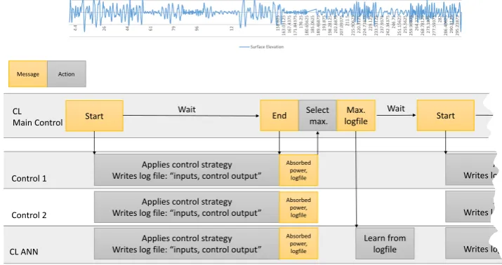
58
The problem of getting an accurate model is tackled in [12] with the help of ANN: The net is trained
59
to mimic the behaviour of a WEC, the so obtained model is then used by a conventional control
60
algorithm to predict the best working state for the real buoy. In [13] an approach is presented that
61
learns "on-the-fly" using a two step approach: An initial network categorizes the sea states and a
62
second evaluates the optimal parameters for each state.
63
In this paper the on-the-fly (or online) learning strategy is adapted to make use of the array
64
configuration in which the energy converter will operate. We extend the supervised learning approach
65
by generating the reference pattern during the learning phase. Therefore two or more energy absorbers,
66
of which at least one has to be controlled by the artificial neural net presented in this paper, have to be
67
placed so that they are effected by the energy medium at the same time. During operation all energy
68
absorbers apply their control strategy and monitor their absorbed energy; the control strategy with the
69
highest energy absorption is then used to train the network.
70
This approach differs from the similar Ensemble learning, as it does not try to find the optimal
71
model for each state, but use it to learn a network.The aim of this approach is to get a single neural
72
network handling all cases, instead of a set of models which are specialized in different fields; this
73
gives a big degree of freedom, as the process is not divided into learning and operating. Also the
74
approach is strictly speaking a multi-agents system, it should be classified as a parallel single-agent
75
system, due to the neglected interactions between the devices.
3 of 15
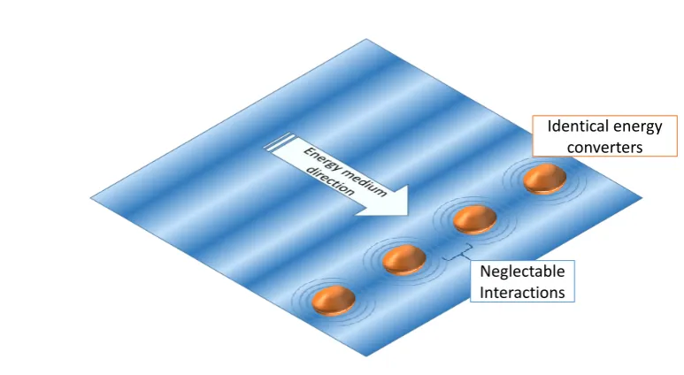
Identical energy converters
Neglectable Interactions
Figure 1.Sketch of an energy converter array that can be used for CL.
As in this strategy several energy converter are helping each other (or at least they help all
77
learnable algorithms in the group) to solve a common task; this paper will refer to this strategy as
78
Collaborative Learning (CL) analogue to the teaching method in schools [14].
79
The CL strategy will be demonstrated on a WEC array (set up see Figure1). WECs are used to
80
extract energy from ocean waves, and are therefore ment to play an important role in providing a
81
sustainable energy source that can be more accurate forecasted than wind and solar energy[15]. From
82
the Edinburgh Duck, one of the earliest and most well known modern WEC, a lot of different designs
83
have been developed, but in general they can be categorized in three types: Attenuator, Point absorber
84
and Terminators [16]. The CL strategy will work for any type as long as it is controllable, however this
85
paper will concentrate on a direct driven point absorber with an electrical linear generator, similar to
86
the devices which are built and operated by Uppsala University on the west coast of Sweden [17]. In
87
contrast to these real existing devices, here it is assumed that the generator damping can be adjusted
88
by choppering the coils [18]. This is a relatively cheap and effective way to control a WEC and may be
89
implemented in existing devices without large modifications.
90
The next chapter starts with the detailed presentation of the collaborative control strategy. It then
91
continues with the description of the physical scale model and the mathemtical model behind the
92
numerical simulation. Chapter 3 is about how the experiments were performed and shows the results,
93
which will then be discussed in the fourth chapter. The last part is an outlook what might be done in
94
the future.
95
2. Methods
96
2.1. Artifical neural networks & Collaborative Learning
97
To focus on the CL strategy instead of the artificial neural network itself, only well established
98
approaches for the network design are used. For systems with temporal dynamic behaviour two
99
network concepts are common in the literature:
100
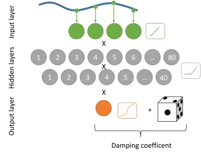
• Recurrent neural networks (RNN), where the connection between units form a directed cycle. A
101
popular subset of RNNs are long-short-term memory networks. For RNN the computational
102
costs are higher than for feed-forward-networks.
103
• In feed forward networks the connection between units can not form a cycle, the information
104
passes only in one direction. To give them the ability to memorize, the input layer has to be
105
extended with units getting a time-delayed input signal.
106
Due to the reduced computational complexity a feed-forward-network is used. The weights were
107
updated using back propagation. For the input, at least one signal has to be related to the amount of
108
currently absorbable energy. The number of units in the input layer depends on the length of the series
109
of previous input values. The output neuron(s) is/are the state(s) of the system that can be controlled.
110
Collaborative learning
111
For training the network uses a special form of supervised learning. In the classic form of
112
supervised learning a teacher knows the correct input and output data. The network changes its
113
internal weights so that the error between network-output and reference data for a specific input
114
pattern decreases. Therefore during the learning process the output error is back-propagated through
115
the network to adjust the weight between the units in all layers.
116
In this case there is no reference data, and it can not even be judged if the output for a given
117
input is beneficial. But there are several energy converters in a row, which are all affected at the same
118
time. With these prerequisites, the approach is to apply different control strategies to each converter, of
119
which at least one is the artificial CL network. The power output and the applied damping are logged
120
for each converter. After a specified time frametset, which consists of several pairs of measured input
121
and applied output data (called a sample), the average energy absorption is calculated. The samples of
122
a converter recorded within this time frame are called a sample set. The sample set of the converter
123
that absorbs the highest amount of power is used to train the neural network. In the following the
124
complete procedure is described step by step:
125
The CL process
126
1. Initial condition: Two or more identical energy converters, all applying different control strategies,
127
of which at least one is the CL network, are placed so that they will be affected by the energy
128
resource at the same time.
129
2. The main program sends the "Start" message to all converters.
130
3. The converters write continuously the sample data (values of the input and output units) in a log
131
file.
132
4. After a time periodtset, the main control sends the "Stop" message to all converters; in return the
133
main program receives all sample sets.
134
5. The CL algorithm calculates the average absorbed power for each converter and chooses the
135
sample set of the converter with the highest absorption.
136
6. This sample set’s input and output is used to train the CL network.
137
7. After the training is finished, the procedure repeats from step 2.
138
The process is visualized in Figure2.
139
The sampling frequencyff as well as the time intervaltsethave to be equal for all converters. If
140
the controller focuses on the short or long term power absorption depends on the sample set duration:
141
A short duration will push the CL-network to maximize the current power absorption, without taking
142
into account if the action that is taken now will also be beneficial for power absorption in the future.
143
Under realistic conditions, the lower limit fortsetis the time the controller needs to apply a specific
144
parameter and get reliable measurements of how this effects the power absorption. Furthermore, when
145
it can not be guaranteed that all converters are effected by the energy source at the same time,tset
146
should be much higher than the time differences between the converters.tsetshould be chosen much
147
smaller than a specific state of the energy resource (for example wind speed, sea state) typically lasts.
148
Evaluation
149
After the learning phase an ANN is evaluated with a second test data set. During the test session,
150
the ANN calculates the output without information about the reference, i. e. without learning. The
151
data is then compared with the reference. Training and test data should be slightly different to evaluate
152
the network’s ability to generalize.
5 of 15
0.4
4.4 26 44 61 79 96 12 158.625 163.03125 167.4375 171.84375
176.25
180.65625 185.0625 189.46875 193.875 198.28125 202.6875 207.09375
211.5
215.90625 220.3125 224.71875 229.125 233.53125 237.9375 242.34375
246.75
251.15625 255.5625 259.96875 264.375 268.78125 273.1875 277.59375
282
286.40625 290.8125 295.21875 Wave Data (over time)
Surface Elevation
Start CL
Main Control
Applies control strategy Writes log file: “inputs, control output” Control 1
Applies control strategy Writes log file: “inputs, control output”
Applies control strategy Writes log file: “inputs, control output” Control 2
CL ANN
End
Absorbed power, logfile
Absorbed power, logfile
Absorbed power, logfile
Select max.
Max. logfile
Learn from logfile
Start
Applies control strategy Writes log file: “inputs, control output”
Applies control strategy Writes log file: “inputs, control output”
Applies control strategy Writes log file: “inputs, control output”
Message Action
Wait Wait
Figure 2.Block diagram of the CL control method.
2.2. Scale model
154
The type of point absorber used in this paper is inspired by the WECs developed by Uppsala
155
University for the Lysekil project [17]. These wave converters consists of three parts: The float, here
156
a cylindrical buoy, the Power-Take-Off (PTO), here an electrical linear generator with adjustable
157
damping, and a line connecting the buoy and PTO, see also Figure3.
158
The translator of the linear generator has a given stroke lengthlT, so that the position of the translatoryhas to be within the limits:
05y5lT.
To protect the mechanical casing, springs with a lengthlcare mounted on the top and bottom to
159
prevent the translator hitting the end stops.
160
In contrast to the real existing generators, the converter used in this work is able to actively change the damping in short term, which is a simple way of controlling the WEC and optimize wave energy absorption for different sea states. For a real generator the dampingγcan only be adjusted within a range:
γmin5γ5γmax.
A load cell is placed between line and translator to measure the force in the line.
161
For collaborative learning two or more devices have to be in line parallel to the wave front. How
162
the interaction between buoys influences the power absorption and optimal damping of WECs in wave
163
farms is a topic of ongoing research, but most studies suggest that the influence is neglectable small if
164
the WECs are in line to the wave front and have sufficient space in-between each other [19]. For now it
165
is assume that the interaction between the WECs in our array will have no significant influence on the
166
optimal damping and absorbed power.
167
2.3. Numerical Model
168
The simulation uses a three body model consisting of buoy, translator and a connecting line. As
169
the control strategy itself does not care about the specific WEC the main goal was to achieve a fast
170
numerical model that captures the relevant behaviour qualitatively rather than a quantitative accurate
171
simulation. Therefore the assumptions of linear potential theory is used, but in contrast to many
172
other numerical models, this approach did not use boundary-integral equations methods (BIEMs) to
173
calculate the hydrodynamic coefficients. Since point absorber have a small surface area, and linear
174
potential theory assumes flat waves, the pressure over the surface can be approximated as constant and
175
the defraction of the waves is neglectable small. Furthermore the only motion of interest is in heave
176
direction. These assumptions lead to a fast, but accurate model, which is not based on convolution
177
terms and therefore causal. In addition this model can account for non-linearities due to the position
178
of the buoy into account, so the model stays valid for large movements, unlike purely linear potential
179
theory based models (compare simulation results in [20]).
180
As no numerical model is able to simulate all aspects of a physical test, the wave tank test is
181
performed in addition to the numerical model focusing on how the algorithm handles measured data.
182
Heave Force
183
The force from the water surface in heave direction is, according to Bernoulli’s principle, made of two forces, the potential forceFBcand the kinetic forceFH. Both depend on the surface elevationhand the buoy’s positionx. For the heave force only the kinetic force is considered, the potential force is included in the buoyancy force. As long as the buoy’s position is in the water and the surface level is rising upwards relative to the buoy’s motion, the heave force is applied.
FH=
(
ABρ(h˙−x˙)2 , x<h∧h˙−x˙ >0
0 , else , (1)
whereρis the density of water andABis the (wetted) area of the buoy parallel to the surface.
184
Buoy
185
The buoy is modelled as a linear mass-spring-damper system which is affected by the heave force FH, the buoyancy forceFBc=ρgAB(h−x), the gravity forceFBg=mBg, withgbeing the gravitational acceleration constant, the hydrodynamic damping forceFbd=dBx˙and the line forceFL. The equation of motion for the buoy is
¨
x= FH+FBc+FBg+Fbd mB+mA ,
withmBbeing the mass andmAbeing the added mass of the buoy, andFbdthe damping of the buoy,
186
motivated by the radiated wave of the buoy.
187
Line
188
The line, modelled as a spring-damper system, is only activated if the distance between buoy and translator is larger than the length of the line.
FL=
(
cR(x−y) +dR(x−y) ,x>y
0 ,else , (2)
withcrbeing the stiffness anddRthe damping of the line.
189
Translator
190
The translator is modelled as a linear mass-damper system, which is affected by the gravity force FTg and the line force FL. The damping force FTd is the product of the damping factorγand the translator’s velocity;γis set by the control algorithm. So the forceFTacting on the translator is:
FT =FTg+FTm+FTd−FL, (3)
withFTg=mTgandFTm=mTy¨;mTis the mass of the translator. Furthermore an end stop forceFStop is introduced which consists of a spring and a position limit. The position limits are at the upper and lower end of the translator. The springs have a length ofls and are positioned at the end stops. They provide the spring forceFTs.
FStop =
(
FTs ,ls>y>0∨lT−ls <y<lT)
7 of 15
Table 1.Parameters
translator mT 6 kg
lT 0.32 m
ls 0.08 m
buoy mB 5 kg
mA 0.3 kg
Sw 0.2 m2
dB 50 Ns/m line dR 84000Nsm
cR 40000Nm
The equation of motion for the translator is:
¨
y= FTg+FTd−FL+FStop mT
. (4)
Parametrisation
191
The parameters of the simulations can be found in Table1. They correspond to a 1:10 scale of the
192
full scale WEC, which is similar to the device used in the wave tank test. The stiffness of the line was
193
limited by the numerical stability of the simulation; the damping in the line was set so that there were
194
no significant oscillations in the line. The added mass and damping of the buoy were chosen to match
195
with data obtained from a decay test with the physical buoy model.
196
2.4. Wave tank model
197
For the wave tank test an ellipsoidal buoy with a diameter of 0.5 m was used, which was connected with a line, guided by a pulley system, to the PTO. The PTO consisted of an electric linear motor that mimics a generator, which enables us to implement nearly all common control strategies. In this paper it is used to simulate a generator with constant damping. So the applied force is proportional to the measured speed of the translator:
FPTO =γy˙.
A more detailed description of the set-up can be found in [4]. The force controller runs with a frequency
198
of 100 Hz.
199
3. Experiments
200
The simulation and the wave tank test were designed to supplement each other. Both use similar
201
1:10 scale buoys and the same neural network. During the simulation the CL algorithm is training
202
along with four constant damping controls.
203
In the tank test only two WECs can run at the same time, which leads to a slightly modified
204
test: The sample sets of two constant damping controlled WECs are recorded and then the winning
205
sampling set is fed to the neural network. This procedure is repeated for the training wave, but at this
206
time, the network is not trained with the sample set but had to predict the winning damping.
207
3.1. Artificial Neural Network
208
The main objective with designing the artificial neural network was to achieve a fast learning
209
process; especially for the experiments in a wave tank noticeable results should be seen in less than
210
one hour. Complex deep networks that have achieved remarkable results in different areas, come with
211
the cost of a long learning process which requires a big training data set. Finding the balance between
212
Surface
Elevation (h)
Calculate the heave force:
F
H=f(p,dx,dw)
H
ea
ve
For
ce
(FH
)
m
buoy
d
c
m
d
tr
ans
la
tor
line
c
c
b
u
o
y
p
osit
ion
(
x)
d
c
The line force is only
active if the line
is under tension
9 of 15
pattern recognizing and fast learning progress, a network with eight hidden layers is chosen as the
213
main network (CL-ANN1). Furthermore a second network (CL-ANN2) was applied in the simulation,
214
using two hidden layers and a random generator, which added a random number to the output, giving
215
it the ability to explore new damping coefficients outside its policy. A sketch of the set-up of both
216
networks can be found in Figure4and5. To speed up the learning process and get the samples sets
217
randomized, each sample set is learned ten times in intervals of a few minutes.
218
The input has to be related to the current wave force acting on the WEC. This could be done by
219
placing a wave measurement buoy in line with the WECs, but with an adequate accuracy the wave
220
force can also be obtained by a load cell measuring the force in the line and subtracting the damping
221
force of the generator. Inertia and wave interaction of the buoy still influence the rope force, but as
222
they are similar for all WECs, it will not influence the learning process of the CL-network.
223
Real surface gravity waves used for wave power have frequencies lower than 0.5 Hz and according
224
to the Nyquist-criteria the sampling frequency should then be higher than 1 Hz. We set it toff =1.5 Hz
225
(full scale). The number of input units was set to 5, as f1
f10=6.67sis a suitable window length. While
226
the first input unit get the current force signal, the second get previous value (delayed by f1
f) and so
227
on.
228
The output of the network is the normalized dampingγout, using the following formula to resize it to its actual valueγ:
γ= (γout(γmax−γmin)) +γmin
A sample set duration was set totset=3s(full scale) in the simulation and totset=6s(full scale) in
229
the wave tank test.
230
As activation function for the hidden layers the ramp (ReLU) is used, which is known to enable
231
fast learning rate over layers [21], and a logistic function is applied for the output units. The bias and
232
weights of all units are set randomly.
233
3.2. Wave data
234
The training wave data used for both - simulations and wave tank tests - is a 10 min (about half
235
an hour in full scale) long medley consisting of 20 Bretschneider spectra sea states ranging from a full
236
scale energy period of 3.5 s to 10.5 s and from a full scale significant wave height of 0.75 m to 3.25 m.
237
The sequence was designed in such a way, that different sea states alternate, but at the same time it
238
was ensured that the sea state will not change abruptly.
239
The test wave sequence is similar to the training data but shorter (3 min, 51 s in 1:10 scale) and
240
consists of eight Bretschneider spectra which were not used during the training period, but are within
241
the same range of energy period and wave height.
242
3.3. Simulation test
243
Two simulations were done, in which the WECs were placed in a row perpendicular to the wave
244
front and all hydrodynamic interactions between the buoys were neglected. The first simulation is
245
called static, as among the five WECs which were simulated only one uses the CL-network; the four
246
other WECs used a static constant damping with 200, 300, 400 and 500 Ns/m.
247
During the second simulation the focus was on the dynamic learning process between two
248
CL-networks. To prevent both networks from doing the same, they were given different ’characters’.
249
The first network (CL-ANN1) is slow learning and looks for the best control strategy in long term
250
while the second network (CL-ANN2) has the task to explore new damping coefficients.
251
All control algorithm are connected and supervised by the main program, that is starting and
252
stopping the recording of the input and output data of each control. Figure8shows the average
253
absorbed power for each WEC during the test sequence.
254
…
…
X
X
120 x 80 x 40 x 80 x
40 x 80 x 80 x 40
H
idd
en
la
yer
s
Output
la
yer
In
pu
t
la
yer
Damping coefficent
Figure 4.Number of layers and neurons for the collaborative learning network 1 (CL-ANN1).
2
3
4
5
6
…
1
2
3
4
5
…
1
H
idd
en
la
yer
s
Output
la
yer
X
X
X
80
40
In
pu
t
la
yer
+
Damping coefficent
11 of 15 ͲϬ͘Ϯϱ ͲϬ͘ϭϱ ͲϬ͘Ϭϱ Ϭ͘Ϭϱ Ϭ͘ϭϱ Ϭ͘Ϯϱ Ϭ ϲ ϭϯ ϭϵ Ϯϱ ϯϭ ϯϴ ϰϰ ϱϬ ϱϲ ϲϯ ϲϵ ϳϱ ϴϭ ϴϴ ϵϰ ϭϬϬ ϭϬϲ ϭϭϯ ϭϭϵ ϭϮϱ ϭϯϭ ϭϯϴ ϭϰϰ ϭϱϬ ϭϱϲ ϭϲϯ ϭϲϵ ϭϳϱ ϭϴϭ ϭϴϴ ϭϵϰ ϮϬϬ ϮϬϲ Ϯϭϯ Ϯϭϵ ϮϮϱ Ϯϯϭ ƐƵ ƌĨ ĂĐ Ğ Ğů Ğǀ Ăƚ ŝŽ Ŷ ŵ ƚŝŵĞƐ ͲϬ͘Ϯϱ ͲϬ͘ϭϱ ͲϬ͘Ϭϱ Ϭ͘Ϭϱ Ϭ͘ϭϱ Ϭ͘Ϯϱ Ϭ ϴ ϭϲ Ϯϯ ϯϭ ϯϵ ϰϳ ϱϱ ϲϯ ϳϬ ϳϴ ϴϲ ϵϰ ϭϬ Ϯ ϭϬ ϵ ϭϭ ϳ ϭϮ ϱ ϭϯ ϯ ϭϰ ϭ ϭϰ ϴ ϭϱ ϲ ϭϲ ϰ ϭϳ Ϯ ϭϴ Ϭ ϭϴ ϴ ϭϵ ϱ ϮϬ ϯ Ϯϭ ϭ Ϯϭ ϵ ϮϮ ϳ Ϯϯ ϰ Ϯϰ Ϯ Ϯϱ Ϭ Ϯϱ ϴ Ϯϲ ϲ Ϯϳ ϯ Ϯϴ ϭ Ϯϴ ϵ Ϯϵ ϳ ϯϬ ϱ ϯϭ ϯ ϯϮ Ϭ ϯϮ ϴ ϯϯ ϲ ϯϰ ϰ ϯϱ Ϯ ϯϱ ϵ ϯϲ ϳ ϯϳ ϱ ϯϴ ϯ ϯϵ ϭ ϯϵ ϴ ϰϬ ϲ ϰϭ ϰ ϰϮ Ϯ ϰϯ Ϭ ϰϯ ϴ ϰϰ ϱ ϰϱ ϯ ϰϲ ϭ ϰϲ ϵ ϰϳ ϳ ϰϴ ϰ ϰϵ Ϯ ϱϬ Ϭ ϱϬ ϴ ϱϭ ϲ ϱϮ ϯ ϱϯ ϭ ϱϯ ϵ ϱϰ ϳ ϱϱ ϱ ϱϲ ϯ ϱϳ Ϭ ϱϳ ϴ ϱϴ ϲ ϱϵ ϰ ϲϬ Ϯ ϲϬ ϵ ϲϭ ϳ ϲϮ ϱ ϲϯ ϯ ϲϰ ϭ ƐƵ ƌĨ ĂĐ Ğ Ğů Ğǀ Ăƚ ŝŽ Ŷ ŵ ƚŝŵĞƐ
Figure 6.Training (above) and test (below) wave data in the applied 1:10 scale
60 80 100 120 140 160 180 200 Damp ing coe ffi cen t [N s/m ] time
Winning damping compared to ANN output during the test wave sequence
Winning damping ANN output
Figure 7.Winning damping of both constant damping controls (orange, solid line) compared to the output for the same input of the ANN (moving average, blue dotted line).To increase readability the ANN output is represented by a moving average of 100 values.
3.7 3.8 3.9 4 4.1 4.2 4.3 4.4 Const. Damping 200 Ns/m Const. Damping 300 Ns/m Const. Damping 400 Ns/m Const. Damping 500 Ns/m
CL-ANN1 CL-ANN1 CL-ANN2
A ver ag e ab sor b ed p ow er [W] 100% 99 .5% 91 .8% 99 .7% 97 .8 % 10 1.3 % 98 .3 %
Figure 8.Average absorbed power for the test wave sequence in the simulations. CL-ANN1 indicates the ‘deep’ ANN, and CL-ANN2 the ‘shallow’ ANN.
3.4. Wave Tank Test
255
The physical test was performed in a 1:10 scale in the Ocean Basin of the COAST laboratory of
256
Plymouth University. The test was limited to two running WECs at the same time. Both WECs used
257
a constant damping control and were connected to the CL main program, which synchronized the
258
recording of the data sets. Instead of learning the CL network online, a log file with the winning data
259
set for each time period was written and used to train the CL network offline. Due to friction in the
260
mechanical system the used dampings were much lower then in the simulation and lay on a very
261
flat part of the logistics function, which was motivation to replace the logistic function for the output
262
neurons of the CL network with the linear function.
263
The same procedure was implemented for the test wave sequence, but instead of learning the
264
network, it was only fed with the input data and had to guess the corresponding damping factor.
265
This method had the disadvantage that the ANN was not active itself, but is a good measure of
266
how well the network handles real world data: In Figure7the winning damping over the test data is
267
plotted in comparison with the ANN output for the same data input.
268
4. Discussion
269
Simulation
270
The model is based on simplified hydrodynamic wave-body interactions. Therefore the magnitude
271
of the in- and output values, the damping factors and the absorbed power, are briefly discussed.
272
The damping factors of the generator leading to the highest power absorptions in the numerical
273
simulation (Figure8) are very high; Previous work [4] suggested much lower optimal damping factors.
274
This may be caused by some inaccurate hydrodynamic parameters (for example underestimation of
275
hydrodynamical damping) due to the simplification made. However the power output is with about
276
4 W in the expected range [4], indicating that the hydrodynamic inaccuracies may have only small
277
influence on the overall performance of the model.
278
Static test
279
At first, the result of the collaborative-learning is compared to the simple constant damping
280
control. According to Figure8, the two best constant damping controls and the CL-network are
281
performing similarly well. The differences are 0.3% and therefore irrelevant. We explain this as the
282
neural network is not strong enough to clearly identify the different sea states; this corresponds to the
283
small variability of the damping coefficients. Instead the CL-network is able to find a good working
284
point for all sea states, that it varies slightly.
285
Dynamic test
286
While the static test shows that the network is able to get the most beneficial damping from
287
existing controls, the dynamic run shows that a group of CL-algorithms is able to find (local) optimums
288
without any a priori information. Moreover, the results in Figure8show that the CL-ANN1 and
289
CL-ANN2 push each other to achieve better results and so absorb even more power than during the
290
dynamic test. The second CL-network is at a disadvantage because of the large exploration factor. In
291
real applications this factor would be much slower; however, in this case a large exploration factor
292
helps to accelerate the learning process. The advantage of the CL-ANN1 control over the constant
293
damping WECs is with 1.6% very small. This must be seen in relation to the influence of the damping
294
factor on the absorbed power: the ratio between the highest and lowest constant damping factor is
295
2.5, but the maximal difference in absorbed power between two constant damping WECs is only 7.9%.
296
Huge differences in power absorption in the evaluation wave sequence are therefore not expected with
297
this WEC type.
13 of 15
Wave tank test
299
During the test under realistic conditions in the wave tank the network showed no problems with
300
handling noisy real world data as can be seen in Figure7. The damping coefficient is fluctuating a bit,
301
but all in all the ANN follows the reference values very well. A fluctuating is not necessarily a bad
302
sign, it shows that the system is not over trained and therefore has not lost its ability to generalize.
303
5. Conclusion Outlook
304
In this paper the CL learning was introduced which is a very flexible way of controlling a converter
305
compared to traditional supervised or ensemble learning strategies: The process does not have to be
306
divided into training and operation state, as it does in traditional supervised or ensemble learning;
307
Instead the learning is done "on the fly" during normal operation.
308
When using several CL-networks with different characteristics, this can lead to a dynamic process,
309
in which the networks will "push" each other to improve the parameters. This control strategy is
310
especially useful in high dynamic environments with interactions between the controlled units.
311
The control did not improve the absorbed power significantly. The artificial neural network used
312
in this model was not strong enough to handle the noisy data and classify the sea states clearly. Ways
313
to tackle this problem could be a very deep network or an algorithm easing the learning process by
314
preprocessing the data; for example by splitting the learning process into wave based sample sets or
315
by analysing the sea state and using wave height and energy period as inputs of the network.
316
Controlling only the damping of an energy converter has a minor influence compared to many
317
other control strategies. This can be noticed in the small differences between the different damping
318
coefficients in Figure8. Especially latching and reactive control can increase the power absorption
319
significantly. To implement the CL network for one of these controls could ease the search for the
320
optimal parameters for the network, compared to the damping control with its very small differences.
321
This paper neglected the interaction between the WECs in line with the wave crest, assuming
322
these will have minor influence on the optimal damping as for example the results of [22] suggest.
323
Further studies could focus on the influence of interaction between WECs - first on the interaction of
324
WECs in a line parallel to the wave, then also interaction between the WECs in several rows.
325
Author Contributions:The general conceptualization and methodology were done by S.T. who also wrote most of
326
the paper. The conceptualization and design of the physical PTO were done by J.E., M.E. and S.T.. The planning of
327
the wave tank experiments were done by M.G. (Marianna Giassi) and S.T. with help of J.E., M.G. (Malin Göteman),
328
E.R. and M.H.. The simulation tool was written by S.T.. M.G. (Marianna Giassi), M. G. (Malin Göteman), J. E.
329
and J.I. were involved in all stages of the project and contributed with ideas and advice. Project administration,
330
including supervision, was done by M.G., J.E. M.E. M.H. and J.I.. M.G., J.E. and J.I. were furthermore responsible
331
for the funding acquisition. All authors contributed to the paper with reviewing and editing.
332
Funding:The authors want to thank the Swedish Energy Agency (project number 40421-1), the Swedish Research
333
Council (VR, grant number 2015-04657) for funding this research and the Åforsk Foundation. This work was
334
supported by Stand Up for Energy.
335
Acknowledgments:This paper would not exist in this form without the help of Oliver Goldsmith, Liz Dunsmoor,
336
Tara Büttner and Keiran Monk during the wave tank test. Furthermore the authors want to thank the Swedish
337
Energy Agency (project number 40421-1), the Swedish Research Council (VR, grant number 2015-04657) and the
338
Åforsk Foundation for funding this research. This work was supported by Stand Up for Energy. The authors
339
declare no conflict of interest.
340
Conflicts of Interest:The authors declare no conflict of interest.
341
Abbreviations
342
The following abbreviations are used in this manuscript:
343 344
ANN Artificial neural network
CL Collaborative learning
CL-ANN1 ‘deep’ ANN used for the learnable WEC CL-ANN2 ‘shallow’ ANN used for the learnable WEC COAST laboratory Coastal, ocean and sediment transport laboratory;
Facility at the University of Plymouth containing the wave tank
PTO Power take-off
WEC Wave energy converter
345
346
1. Salter, S.; Jeffery, D.; Taylor, J. The architecture of nodding duck wave power generators.The Naval Archtiect
347
1976, pp. 21–24.
348
2. Li, G.; Belmont, M.R. Model predictive control of sea wave energy converters - Part I: A convex approach
349
for the case of a single device.Renewable Energy2014,69, 453 – 463.
350
3. Soliman, M.; Malik, O.P.; Westwick, D.T. Multiple Model Predictive Control for Wind Turbines With
351
Doubly Fed Induction Generators. IEEE Transactions on Sustainable Energy2011,2, 215–225.
352
4. Thomas, S.; Giassi, M.; Göteman, M.; Eriksson, M.; Isberg, J.; Engström, J. Optimal Constant Damping
353
Control of a Point Absorber with Linear Generator In Different Sea States: Comparision of Simulation and
354
Scale Test. 12th European Wave and Tidal Energy Conference, Cork, Ireland, 2017.
355
5. Fusco, F.; Ringwood, J.V. A Simple and Effective Real-Time Controller for Wave Energy Converters. IEEE
356
Transactions on Sustainable Energy2013,4, 21–30.
357
6. Barrett, D.S.; Triantafyllou, M.S.; Yue, D.K.P.; Grosenbaugh, M.A.; Wolfgang, M.J. Drag reduction in
358
fish-like locomotion. Journal of Fluid Mechanics1999,392, 183–212. doi:10.1017/S0022112099005455.
359
7. Hinton, G.; Deng, L.; Yu, D.; Dahl, G.E.; r. Mohamed, A.; Jaitly, N.; Senior, A.; Vanhoucke, V.;
360
Nguyen, P.; Sainath, T.N.; Kingsbury, B. Deep Neural Networks for Acoustic Modeling in Speech
361
Recognition: The Shared Views of Four Research Groups.IEEE Signal Processing Magazine2012,29, 82–97.
362
doi:10.1109/MSP.2012.2205597.
363
8. Krizhevsky, A.; Sutskever, I.; Hinton, G.E. ImageNet Classification with Deep Convolutional Neural
364
Networks. InAdvances in Neural Information Processing Systems 25; Pereira, F.; Burges, C.J.C.; Bottou, L.;
365
Weinberger, K.Q., Eds.; Curran Associates, Inc., 2012; pp. 1097–1105.
366
9. Silver, D.; Huang, A.; Maddison, C.J.; Guez, A.; Sifre, L.; van den Driessche, G.; Schrittwieser, J.;
367
Antonoglou, I.; Panneershelvam, V.; Lanctot, M.; Dieleman, S.; Grewe, D.; Nham, J.; Kalchbrenner,
368
N.; Sutskever, I.; Lillicrap, T.; Leach, M.; Kavukcuoglu, K.; Graepel, T.; Hassabis, D. Mastering the Game of
369
Go with Deep Neural Networks and Tree Search.Nature2016,529, 484–489. doi:10.1038/nature16961.
370
10. Ng, A.Y.; Coates, A.; Diel, M.; Ganapathi, V.; Schulte, J.; Tse, B.; Berger, E.; Liang, E., Autonomous Inverted
371
Helicopter Flight via Reinforcement Learning. InExperimental Robotics IX: The 9th International Symposium
372
on Experimental Robotics; Ang, M.H.; Khatib, O., Eds.; Springer Berlin Heidelberg: Berlin, Heidelberg, 2006;
373
pp. 363–372. doi:10.1007/11552246\_35.
374
11. Mundon, T.R.; Murray, A.F.; Hallam, J.; Patel, L.N., Causal Neural Control of a Latching Ocean Wave
375
Point Absorber. InArtificial Neural Networks: Formal Models and Their Applications – ICANN 2005: 15th
376
International Conference, Warsaw, Poland, September 11-15, 2005. Proceedings, Part II; Duch, W.; Kacprzyk,
377
J.; Oja, E.; Zadro ˙zny, S., Eds.; Springer Berlin Heidelberg: Berlin, Heidelberg, 2005; pp. 423–429.
378
doi:10.1007/11550907underline67.
379
12. Beirao, P.; Mendes, M.; Valério, D.; da Costa, J.S. Control of the archimedes wave swing using neural
380
networks. 7th European Wave and Tidal Energy Conference, 2007.
381
13. Anderlini, E.; Forehand, D.; Bannon, E.; Abusara, M. Reactive control of a wave energy converter
382
using artificial neural networks. International Journal of Marine Energy 2017, 19, 207 – 220.
383
doi:https://doi.org/10.1016/j.ijome.2017.08.001.
384
14. Gokhale, A. Collaborative Learning Enhances Critical Thinking. Journal of Technology Education1995,
385
7, 22–30.
386
15. Reikard, G.; Robertson, B.; Bidlot, J.R. Combining wave energy with wind and solar: Short-term forecasting.
387
Renewable Energy2015,81, 442 – 456. doi:http://doi.org/10.1016/j.renene.2015.03.032.
15 of 15
16. Drew, B.; Plummer, A.R.; Sahinkaya, M.N. A review of wave energy converter technology. Proceedings
389
of the Institution of Mechanical Engineers, Part A: Journal of Power and Energy 2009, 223, 887–902,
390
[https://doi.org/10.1243/09576509JPE782]. doi:10.1243/09576509JPE782.
391
17. Lejerskog, E.; Gravråkmo, H.; Savin, A.; Strömstedt, E.; Tyrberg, S.; Haikonen, K.; Krishna, R.; Boström, C.;
392
Rahm, M.; Ekström, R.; Svensson, O.; Engström, J.; Ekergård, B.; Baudoin, A.; Kurupath, V.; Hai, L.; Li, W.;
393
Sundberg, J.; Waters, R.; Leijon, M. Lysekil Research Site, Sweden : A status update. 9th European Wave
394
and Tidal Energy Conference, Southampton, UK, 2011, 2011.
395
18. Ekström, R.; Ekergård, B.; Leijon, M. Electrical damping of linear generators for wave energy converters
-396
A review.Renewable and Sustainable Energy Reviews2015,42, 116 – 128.
397
19. Borgarino, B.; Babarit, A.; Ferrant, P. Impact of wave interactions effects on energy
398
absorption in large arrays of wave energy converters. Ocean Engineering 2012, 41, 79 – 88.
399
doi:https://doi.org/10.1016/j.oceaneng.2011.12.025.
400
20. Clément, A.H.; Babarit, A. Discrete control of resonant wave energy devices. Philosophical Transactions
401
of the Royal Society of London A: Mathematical, Physical and Engineering Sciences 2011, 370, 288–314.
402
doi:10.1098/rsta.2011.0132.
403
21. Glorot, X.; Bordes, A.; Bengio, Y. Deep Sparse Rectifier Neural Networks. Proceedings of the Fourteenth
404
International Conference on Artificial Intelligence and Statistics; Gordon, G.; Dunson, D.; Dudík, M., Eds.;
405
PMLR: Fort Lauderdale, FL, USA, 2011; Vol. 15,Proceedings of Machine Learning Research, pp. 315–323.
406
22. Nambiar, A.J.; Forehand, D.I.; Kramer, M.M.; Hansen, R.H.; Ingram, D.M. Effects of hydrodynamic
407
interactions and control within a point absorber array on electrical output. International Journal of Marine
408
Energy2015,9, 20 – 40. doi:https://doi.org/10.1016/j.ijome.2014.11.002.
409