The Tsallis Distribution at the LHC

The Tsallis Distribution at the LHC

Jean Cleymans1

1_{UCT-CERN Research Centre and Department of Physics} University of Cape Town, Rondebosch, South Africa

Abstract. The Tsallis distribution has been used widely in high energy physics to de-scribe the transverse momentum distributions of particles. In this note we show that the use of a thermodynamically consistent form of this distribution leads to a description of identified particles with the same values of the temperatureTand the parameterq.

There exists a rich and wide variety of distributions covering a large range of applications [1, 2]. Those having a power law behaviour have attracted considerable attention in physics in recent years but there is a a long history in other fields such as biology and economics [3].

In high energy physics power law distributions have been applied by a very large number of scientists [4–8] to the description of transverse momenta of secondary particles produced in p−p collisions. Indeed the available range of transverse momenta has expanded considerably with the advent of the Large Hadron Collider (LHC). Collider energies up to 8 TeV are now available inp−p collisions and transverse momenta of hundreds of GeV are a common occurrence. In this presentation the focus will be on various forms of distributions first proposed by C. Tsallis about twenty-five years ago [9].

In the analysis of the new data, a Tsallis-like distribution gives excellent fits to the transverse momentum distributions as shown by the by the ALICE [6], ATLAS [7] and CMS [8] collaborations at the LHC and by the STAR [4] and PHENIX [5] collaborations at RHIC. In this paper we review the parameterization used by these groups and propose a slightly different one which has a more consistent interpretation and has the bonus of being thermodynamically consistent.

For high energy physics a consistent form of Tsallis statistics (see e.g. [10] and references therein) for the particle number, energy density and pressure is given by the expressions given below

N = gV

d3_p

(2π)3

1+(q−1)E−μ T − q q−1 , (1) = g

d3_p

(2π)3E

1+(q−1)E−μ T

− q q−1

, (2)

P = g

d3_p

(2π)3

p2

3E

1+(q−1)E−μ T

− q q−1

. (3)

whereT andμare the temperature and the chemical potential,Vis the volume andgis the degeneracy factor. As is well-known the Tsallis distribution [9, 11] introduces a new parameterq which for transverse momentum spectra is always close to 1, typical values for the parameterqobtained are in the range 1.1 to 1.2. In the remainder of this paper we will always assumeq>1.

DOI: 10.1051/ C

Owned by the authors, published by EDP Sciences, 2014 /2014 007 0

The expressions (1), (2) and (3) are thermodynamically consistent, e.g. it can be easily shown [10] that relations of the type

N=V ∂_∂μP

T

, (4)

are satisfied [10, 12]. Note that without the extra power ofqin the equations (1),(2), (3) the thermo-dynamic consistency would not be achieved.

It follows from (1) that the momentum distribution is given by,

d3_N

d3_p =

gV (2π)3

1+(q−1)E−μ T

−q/(q−1)

, (5)

or, expressed in terms of transverse momentum,pT, transverse mass,mT, and rapidityy

d2_N

dpTdy =

gVpTmTcoshy (2π)2

1+(q−1)mTcoshy−μ T

₋q/(q−1)

, (6)

At mid-rapidityy=0 and for zero chemical potentialμ=0 this reduces to

d2_N

dpTdy

_y=0 =g_VpTmT

(2π)2

1+(q−1)mT T

−q/(q−1)

. (7)

This is the expression used in [10, 12] to fit the LHC transverse momentum spectra.

It is well-known since 1988 [9] that in the limit where the parameterqgoes to 1 Eq. (6) reduces to the standard Boltzmann distribution:

lim

q→1

d2_N

dpT dy =

g_VpTmTcoshy

(2π)2 exp

−mTcoshy−μ

T . (8)

The parameterization given in Eq. (7) is close to the one used (but different) e.g. by the ALICE [6], ATLAS [7], CMS [8], STAR [4] and PHENIX [5] collaborations where the following form is used :

d2_N

dpTdy =pT

dN dy

(n−1)(n−2) nC(nC+m0(n−2))

1+mT−m0 nC

−n

(9)

wheren,Candm0are fit parameters. Indeed, after substituting

n→ q

q−1 (10)

and

nC→ T+m0(q−1)

p−p 900 GeV

Particle q T

π+ _{1.154±0.036 0.0682±0.0026}

π− _{1.146±0.036 0.0704±0.0027} K+ 1.158±0.142 0.0690±0.0223 K− 1.157±0.139 0.0681±0.0217 K0

S 1.134±0.079 0.0923±0.0139

p 1.107±0.147 0.0730±0.0425 ¯

p 1.106±0.158 0.0764±0.0464 Λ 1.114±0.047 0.0698±0.0148 Ξ− _{1.110±0.218 0.0440±0.0752}

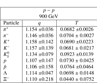
Table 1.Fitted values of theTandqparameters measured inp−pcollisions by the ALICE and CMS collaborations using the Tsallis form (7) for the momentum distribution.

Which, at mid-rapidityy=0 and zero chemical potential, has the same dependence on the transverse momentum as (7) apart from an additional factor mT on the right-hand. It has to be pointed out

explicitly that the inclusion of the rest mass in the substitution Eq. (11) is not in agreement with the Tsallis distribution as it breaksmT scaling which is present in the Tsallis form (6) but not in Eq. (9).

The inclusions of the factormTleads to a more consistent interpretation of the variablesqandT [10,

12].

The distribution (7) has been used to fit the data for identified particles,π,Kandpfor the ALICE [6] collaboration andK0

s,ΛandΞfor the CMS [8] collaboration inp−pcollisions at 900 GeV [10, 12].

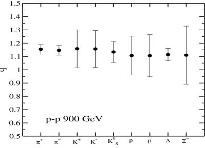
The results are shown in Table 1 for the parametersT andq. The coresponding transverse momentum distributions for the ALICE [6] are shown in Fig. (1). For all identified particles the results are consistent with having a system at a Tsallis freeze-out temperature of about

T ≈70 MeV (13)

and a value for theqparameter of about

q≈1.15 (14)

These values are comparable to the ones obtained recently in [13, 14] where the original proposal of Hagedorn [15] was extended to a Hagedorn-Tsallis distribution.

The consistency of the values ofqis shown in Fig. (2).

0

0.5

1

1.5

2

2.5

3

p

(GeV/c)

0.0001

0.001

0.01

0.1

1

10

dN/dydp

T

π

K

p

0.5

0.6

0.7

0.8

0.9

1

1.1

1.2

1.3

1.4

1.5

q

π+ π− K+ K- K0_S p p Λ _Ξ−

p-p 900 GeV

References

[1] M.E.J. Newman, Contemporary Physics46, 323 (2005).

[2] A. Clauset, C.R. Shalizi, M.E.J. Newman, SIAM Review51, 661, 2009. [3] M. Mitzenmacher, Internet Mathematics,1, 226 (2003).

[4] B. I. Abelev et al. (STAR Collaboration), Phys. Rev. C75, 064901 (2007).

[5] A. Adare et al. (PHENIX Collaboration), Phys. Rev. C83, 052004, (2010); Phys. Rev. C 83, 064903 (2011).

[6] K. Aamodt, et al. (ALICE Collaboration), Eur. Phys. J. C711655 (2011). [7] G. Aad, et al. (ATLAS Collaboration), New J. Phys.13(2011) 053033. [8] V. Khachatryan, et al. (CMS Collaboration), JHEP05, 064 (2011). [9] C. Tsallis, J.Statist.Phys.52, 479 (1988).

[10] J. Cleymans and D. Worku, Eur. Phys. J.A(to be published), arXiv:1203.4343. [11] C. Tsallis, R. S. Mendes, A. R. Plastino, Physica A261, 534 (1998).

[12] J. Cleymans and D. Worku, J. Phys.G39 025006 (2012) . [13] A. Deppman, Physica A391, 6380 (2012).

[14] I. Sena, A. Deppman, arXiv:1208.2952.