A Clutter Suppression Method Based on Improved Principal
Component Selection Rule for Ground Penetrating Radar
Jichao Zhu, Wei Xue*, Xia Rong, and Yunyun Yu
Abstract—Principal component analysis is usually used for clutter suppression of ground penetrating
radar, but its performance is influenced by the selection of main components of target signal. In the paper, an improved principal component selection rule is proposed for selecting the main components of target signal. In the method, firstly difference spectrum of singular value is used to extract direct wave and strong target signal, and then, Fuzzy-C means clustering algorithm is used to determine the weights of principal component of weak target signal. Finally, the principal components of strong target signal and weak target signal are reconstructed to obtain target signal. Experimental results show that the proposed method can effectively remove the clutter signals and reserve more target information.
1. INTRODUCTION
Ground Penetrating Radar (GPR) is an effective tool for underground detection [1, 2] with convenient operation, high resolution and non-destructiveness, and it is widely used in various fields such as civil engineering, archaeology, geology and military. GPR data consist of target and clutter(direct wave, underground clutter and other noise signals) [3–5]. It is difficult to extract target signal especially in the shallow subsurface. Therefore, clutter suppression is an important task for target detection of GPR. Several methods have been applied to clutter suppression in GPR, and among them are clutter model-based methods [6–8], transform domain methods [9–12] and subspace projection methods [13– 17]. Principal Component Analysis (PCA) is a major subspace projection method [14, 15, 18–22], and the main problem of PCA is how to select the principal components of target. An auto-selected rule based on PCA is proposed in [20], and the defect of the method is that threshold selection depends on experiences, which restricts the application of the method. A method based on SVD and Fuzzy-C Means (FCM) is proposed in [22], but FCM is sensitive to single extreme point which causes the degradation of clutter suppression performance.
To solve the problem of extracting weak target signal for point target detection, an improved principal component selection rule based on difference spectrum of singular value and FCM is proposed in the paper. Firstly, difference spectrum of singular value is used to determine the principal component range of direct wave and strong target signal, and then, FCM is applied to the remaining singular values to obtain the principal component weights of weak target signal. Finally, the target signal is reconstructed with principal components of strong target signal and weighted principal components of weak target signal. Some experiments in the case of near field have been executed to evaluate the performance of the proposed method. The experimental results show that the proposed method can remove clutter effectively and reserve more target information.
Received 29 October 2016, Accepted 24 December 2016, Scheduled 6 January 2017
* Corresponding author: Wei Xue ([email protected]).
2. PRINCIPLE OF CLUTTER SUPPRESSION BASED ON PCA
PCA is a linear transformation algorithm based on least mean square error, and it gets orthogonal principal component of signal by special orthogonal matrix. SVD is usually used to implement orthogonal decomposition in PCA, and the signal component corresponding to different singular value is called principal component. Therefore, the selection of the principal component is actually the selection of its corresponding singular value.
B-scan data of GPR can be represented by matrixX∈RM×N, whereM andN are sample numbers for space and time, respectively. According to the composition of GPR data, X can be expressed as:
X=XD +XS+XC (1)
whereXD is the direct wave,XS the target signal, andXC the interference signal (underground clutter and other noise signals).
The SVD ofX can be expressed as:
X=USVT (2)
where U ∈ RM×M and V ∈ RN×N are unitary matrix. S = diag(σ1, σ2, . . . , σr), σi represents the
singular value of X with σ1 ≥ σ2 ≥ . . . ≥ σr ≥ 0, and r is the smaller value of M and N. ui is the
M×1 vector andvi theN×1 vector. Therefore,
X=u1σ1vT1 +u2σ2vT2 +. . .+urσrvrT (3)
Different signal components are reflected by different singular values. The greater singular value corresponds to the signal component with higher energy. The clutter suppression based on PCA firstly determines the singular values of target signal, and then the target signal is reconstructed with its corresponding singular values. In GPR data, the energy ofXD is larger, the energy ofXSin the middle and the energy of XC smaller, so the reconstructed target signal can be given by:
XS =
k2
i=k1
uiσiviT (4)
where k1 to k2 are the subscripts of singular value (1≤k1 ≤k2 ≤r), and the singular values from k1
to k2 belong to target signal.
3. IMPROVED PRINCIPAL COMPONENT SELECTION RULE
3.1. FCM Algorithm
FCM is a clustering algorithm based on partition. In FCM algorithm, the objects belonging to same cluster have the largest similarity, and different clusters have the smallest similarity by minimizing the objective function [23–25]. If the sample A= (a1, a2, . . . , an) is divided into c clusters (T1, T2, . . . , Tc)
by FCM algorithm, the objective functionJF CMm (E,P) is:
JF CMm (E,P) =
n
i=1 c
j=1
emijd2ij (5)
whereE={eij}n×c is the membership matrix, andeij represents membership of specimen ai to cluster
Tj and satisfies cj=1eij = 1, eij ≥ 0,∀i = 1,2, . . . , n. P = (p1, p2, . . . , pc) is the cluster center,
m ∈ [1,∞) the weighted exponent, and the optimal range is (1.5,2.5). dij = ai −pj is Euclidean
distance of specimen ai and cluster centerpj.
The aim of clustering is to obtain the minimum value of the function JF CMm (E,P). Two optimal iterative formulas resulting from Lagrange multiplier theory are given by:
eij = c 1
k=1
dij
dik
2
m−1
pj =
i=1
emij ×ai
n
i=1
emij
j = 1,2, . . . , c (7)
If the two adjacent iterative objective functions satisfy|Jt−Jt+1|< ε, the iteration will stop. εis
the allowable error, and it is a small positive number.
3.2. Principal Component Selection Rule Based on Difference Spectrum and FCM
Since the singular value is in descending order, the energy of its corresponding signal component is also in descending order. Direct wave has strong horizontal correlation and greater energy, and it corresponds to the first few larger singular values. The energy of target decreases as the distance between target and antenna increases. When target and antenna are far apart, the energy of target is close to the energy of underground clutter and interference signals, and it is difficult to extract the weak target signal from echo signal. In order to solve this problem, an improved principle component selection rule based on difference spectrum and FCM is proposed in the paper.
Generally, the singular value of direct wave is much larger than that of target and interference signals, so there is an abrupt change in the singular value curve, and here the difference spectrum of singular value is used to describe the change and defined as:
q=σi−σi+1 i= 1,2, . . . , r−1 (8)
The curve describes the variation between two adjacent singular values, and a peak will occur at the position of abrupt of singular values. If the position of peak is k1, the reconstructed direct wave
can be given by:
XD =
k1
i=1
uiσivTi (9)
For the remainingr−k1 singular values, target signal can be obtained through the combination of
difference spectrum and FCM. For two adjacent values (qk, qk+1) in the remaining difference spectrum
curve, the position relationship between k in the remaining difference spectrum curve and k2 in the
whole difference spectrum is:
k2=k+k1 (10)
When|qk−qk+1|reaches the maximum value, the singular values from the position k1+ 1 to k2 is
considered to correspond to strong target signal, then the strong target signal can be given by:
XSstrong = k2
i=k1+1
uiσivTi (11)
Finally, FCM is used to divide the remaining singular values (σk2+1, σk2+2, . . . , σr) into two clusters.
One cluster is the weak target, and the other is interference signal. According to Equation (5), the objective function is:
JF CMm (E,P) =
r
i=k2+1 2
j=1
emijd2ij (12)
The two iterative formulas are:
eij = 2 1
k=1
dij
dik
2
m−1
pj =
r
i=k2+1
emij ×σi
r
i=k2+1
emij
j = 1,2 (14)
The weak target signal is given by weighted sum of signal components:
XSweak =
r
i=k2+1
ei1uiσivTi (15)
Hence the total target signal can be given by:
XS =XSstrong +XSweak =
k2
i=k1+1
uiσivTi + r
i=k2+1
ei1uiσivTi (16)
4. EXPERIMENTAL VERIFICATION
Simulation data and real GPR data in the case of near field have been applied to evaluate the performance of the proposed method, auto-selected rule based on PCA [20] and FCM based on SVD [22]. Meanwhile, image entropy is used to estimate the clutter suppression performance of the three methods. The image entropy is defined as:
Q= ⎛ ⎝M
i=1 N
j=1
X2(i, j) ⎞ ⎠
2
M
i=1 N
j=1
X4(i, j)
(17)
Image entropy represents the information capacity of image, smaller entropy represents better clutter suppression performance.
4.1. Simulation Data
Simulation data are generated by GPRmax simulator based on finite difference time domain (FDTD) method. The center frequency of antenna is 900 MHz, and the target is a perfectly conducting rebar with 0.05 m diameter and buried at the depth of 0.22 m. The medium is a homogenous medium (εr = 3.0,
σ= 0.01 S/m). The B-scan data contain 82 A-scans, and each A-scan contains 1696 samples.
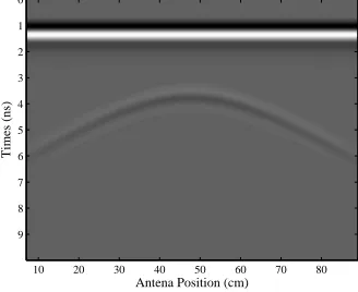
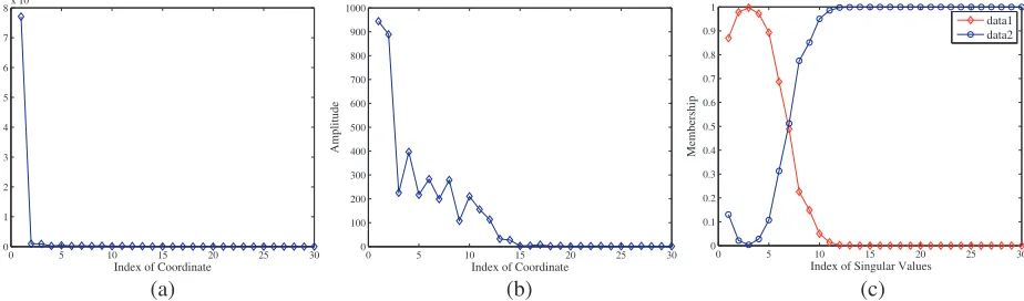
Figure 1 shows the original GPR data in ideal condition, and Figure 2 shows the difference spectrum curve and membership curve of the GPR data. For the proposed method, it can be seen that the strong target signal corresponds to the second and third singular values from Figure 2(a) and Figure 2(b). The fourth and later singular values are clustered by FCM. Figure 2(c) shows the membership function curve. The curve of data1 represents the membership of target signal, and the curve of data2 represents the membership of interference signals.
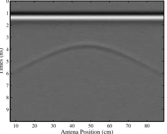
Figure 3(a) shows auto-selected rule based on PCA produces obvious underground clutter. Figure 3(b) shows FCM based on SVD eliminates clutter to a certain extent. Figure 3(c) shows that the proposed method obtains least clutter on the top of the hyperbola, and the edge of the curve is clear. Table 1 shows that the proposed method obtains the smallest entropy under ideal condition. Therefore, the proposed method achieves better clutter suppression performance than other two methods under ideal condition.
Antena Position (cm)
Times (ns)
10 20 30 40 50 60 70 80 0
1 2 3 4 5 6 7 8 9
Figure 1. Original image of simulation data (ideal condition).
0 5 10 15 20 25 30
0 1 2 3 4 5 6 7 8x 10
4
Index of Coordinate
Amplitude
0 5 10 15 20 25 30
0 100 200 300 400 500 600 700 800 900 1000
Index of Coordinate
Amplitude
0 5 10 15 20
0 0.1 0.2 0.3 0.4 0.5 0.6 0.7 0.8 0.9 1
Index of Singular Values
Membership
data1 data2
(a) (b) (c)
Figure 2. Difference spectrum curve and membership curve of simulation data (ideal condition). (a)
Difference spectrum curve of singular value. (b) Difference spectrum curve of singular value without direct wave. (c) Membership function curve.
Antena Position (cm)
Times (ns)
10 20 30 40 50 60 70 80 0
1
2
3
4
5
6
7
8
9
Antena Position (cm)
Times (ns)
10 20 30 40 50 60 70 80 0
1
2
3
4
5
6
7
8
9
Antena Position (cm)
Times (ns)
10 20 30 40 50 60 70 80 0
1
2
3
4
5
6
7
8
9
(a) (b) (c)
Figure 3. Experimental results of simulation data (ideal condition). (a) Auto-selected rule based on
PCA. (b) FCM based on SVD. (c) Proposed method.
Table 1. Entropy comparison of simulation data.
Methods simulation data
ideal condition SNR = 30 dB SNR = 10 dB SNR = 3 dB Auto-selected rule based on PCA 6707.0 6878.1 44278 46019
FCM based on SVD 6588.4 6632.4 42042 44756 Proposed Method 6421.8 6616.1 40851 44737
Antena Position (cm)
Times (ns)
10 20 30 40 50 60 70 80 0
1 2 3 4 5 6 7 8 9
Figure 4. Original image of simulation data with noise (SNR = 30 dB).
0 5 10 15 20 25 30 0
1 2 3 4 5 6 7 8x 10
4
Index of Coordinate
Amplitude
0 5 10 15 20 25 30 0
100 200 300 400 500 600 700 800 900 1000
Index of Coordinate
Amplitude
0 5 10 15 20 25 30 0
0.1 0.2 0.3 0.4 0.5 0.6 0.7 0.8 0.9 1
Index of Singular Values
Membership
data1 data2
(a) (b) (c)
Figure 5. Difference spectrum curve and membership curve of simulation data with noise (SNR =
30 dB). (a) Difference spectrum curve of singular value. (b) Difference spectrum curve of singular value without direct wave. (c) Membership function curve.
Antena Position (cm)
Times (ns)
10 20 30 40 50 60 70 80 0
1
2
3
4
5
6
7
8
9
Antena Position (cm)
Times (ns)
10 20 30 40 50 60 70 80 0
1
2
3
4
5
6
7
8
9
Antena Position (cm)
Times (ns)
10 20 30 40 50 60 70 80 0
1
2
3
4
5
6
7
8
9
(a) (b) (c)
Figure 6. Experimental results of simulation data with noise (SNR = 30 dB). (a) Auto-selected rule
Antena Position (cm)
Times (ns)
10 20 30 40 50 60 70 80 1
2 3 4 5 6 7 8 9
Figure 7. Original image of simulation data with noise (SNR = 10 dB).
0 5 10 15 20 25 30
0 1 2 3 4 5 6 7 8x 10
4
Index of Coordinate
Amplitude
0 5 10 15 20 25 30
0 100 200 300 400 500 600 700 800
Index of Coordinate
Amplitude
0 10 20 30 40 50 60
0 0.1 0.2 0.3 0.4 0.5 0.6 0.7 0.8 0.9 1
Index of Singular Values
Membership
data1 data2
(a) (b) (c)
Figure 8. Difference spectrum curve and membership curve of simulation data with noise (SNR =
10 dB). (a) Difference spectrum curve of singular value. (b) Difference spectrum curve of singular value without direct wave. (c) Membership function curve.
Antena Position (cm)
Times (ns)
10 20 30 40 50 60 70 80 0
1
2
3
4
5
6
7
8
9
Antena Position (cm)
Times (ns)
10 20 30 40 50 60 70 80 0
1
2
3
4
5
6
7
8
9
Antena Position (cm)
Times (ns)
10 20 30 40 50 60 70 80 0
1
2
3
4
5
6
7
8
9
(a) (b) (c)
Figure 9. Experimental results of simulation data with noise (SNR = 10 dB). (a) Auto-selected rule
based on PCA. (b) FCM based on SVD. (c) Proposed method.
Antena Position (cm)
Times (ns)
10 20 30 40 50 60 70 80 0
1 2 3 4 5 6 7 8 9
Figure 10. Original image of simulation data with noise (SNR = 3 dB).
0 5 10 15 20 25 30
0 1 2 3 4 5 6 7 8x 10
4
Index of Coordinate
Amplitude
0 5 10 15 20 25 30
0 50 100 150 200 250 300
Index of Coordinate
Amplitude
0 10 20 30 40 50 60
0 0.1 0.2 0.3 0.4 0.5 0.6 0.7 0.8 0.9 1
Index of Singular Values
Membership
data1 data2
(a) (b) (c)
Figure 11. Difference spectrum curve and membership curve of simulation data with noise (SNR =
3 dB). (a) Difference spectrum curve of singular value. (b) Difference spectrum curve of singular value without direct wave. (c) Membership function curve.
Antena Position (cm)
Times (ns)
10 20 30 40 50 60 70 80 0
1
2
3
4
5
6
7
8
9
Antena Position (cm)
Times (ns)
10 20 30 40 50 60 70 80 0
1
2
3
4
5
6
7
8
9
Antena Position (cm)
Times (ns)
10 20 30 40 50 60 70 80 0
1
2
3
4
5
6
7
8
9
(a) (b) (c)
Figure 12. Experimental results of simulation data with noise (SNR = 3 dB). (a) Auto-selected rule
based on PCA. (b) FCM based on SVD. (c) Proposed method.
4.2. Real GPR Data
Antena Position (cm)
Time (ns)
0 10 20 30 40 50 60 70 80 90 2
4
6
8
10
12
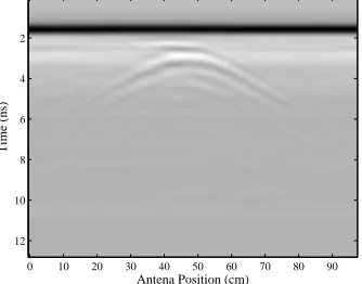
Figure 13. Original image of real GPR data.
0 5 10 15 20 25 30
0 1 2 3 4 5 6 7 8 9 10x 10
5
Index of Coordinate
Amplitude
0 5 10 15 20 25 30
0 0.5 1 1.5 2 2.5 3 3.5
4x 10 4
Index of Coordinate
Amplitude
0 5 10 15 20
0 0.1 0.2 0.3 0.4 0.5 0.6 0.7 0.8 0.9 1
Index of Singular Values
Membership
data1 data2
(a) (b) (c)
Figure 14. Difference spectrum curve and membership curve of real GPR data. (a) Difference spectrum
curve of singular value. (b) Difference spectrum curve of singular value without direct wave. (c) Membership function curve.
Antena Position (cm)
Time (ns)
0 10 20 30 40 50 60 70 80 90 2
4
6
8
10
12
Antena Position (cm)
Time (ns)
0 10 20 30 40 50 60 70 80 90 2
4
6
8
10
12
Antena Position (cm)
Time (ns)
0 10 20 30 40 50 60 70 80 90 2
4
6
8
10
12
(a) (b) (c)
Figure 15. Experimental results of real GPR data. (a) Auto-selected rule based on PCA. (b) FCM
based on SVD. (c) Proposed method.
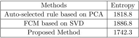
Table 2. Entropy comparison of real GPR data.
Methods Entropy Auto-selected rule based on PCA 1818.8
FCM based on SVD 1886.8 Proposed Method 1742.3
the proposed method obtains lowest entropy among the three methods, which further demonstrates that the proposed method can improve the performance of clutter suppression.
5. CONCLUSION
PCA is an effective method for clutter suppression of GPR, and its performance is influenced by the selection of target principal component. In order to solve the problem of extracting the weak target signal for point target detection, an improved principal component selection rule based on difference spectrum of singular value and FCM is proposed in the paper. The principal components of strong target signal and the weight of principal components of weak target signal are determined by difference spectrum and FCM respectively. The target signals are obtained by reconstructing principal components of strong target signal and weighted principal components of weak target signal. The experimental results show that the proposed method exhibits better clutter suppression performance than other two principal component selection rules.
ACKNOWLEDGMENT
The work is supported by the National Natural Science Foundation of China (Nos. 61401409, 61503351, 61503350) and Hubei province Natural Science Foundation of China (No. 2015CFB520).
REFERENCES
1. Daniels, D. J., Surface-Penetrating Radar, 2nd edition, IEEE Press, 2004.
2. Jol, H. M., Ground Penetrating Radar: Theory and Applications, Elsevier Science, Amsterdam, 2009.
3. Chen, C. S. and Y. Jeng, “Nonlinear data processing method for the signal enhancement of GPR data,” Journal of Applied Geophysics, Vol. 75, No. 1, 113–123, 2011.
4. Soldovieri, F., I. Catapano, P. M. Barone, S. E. Lauro, E. Mattei, E. Pettinelli, G. Valerio, D. Comite, and A. Galli, “GPR estimation of the geometrical features of buried metallic targets in testing conditions,” Progress In Electromagnetics Research B, Vol. 49, 339–362, 2013.
5. Yavuz, M. E., A. E. Fouda, and F. L. Teixeira, “GPR signal enhancement using sliding-window space-frequency matrices,”Progress In Electromagnetics Research, Vol. 145, No 2, 1–10, 2014. 6. Brunzell, H., “Detection of shallowly buried objects using impulse radar,” IEEE Trans. Geosci.
Remote Sens., Vol. 37, No. 2, 875–886, March 1999.
7. Brooks, J. W., L. M. V. Kempen, and H. Sahli, “Primary study in adaptive clutter reduction and buried minelike target enhancement from GPR data,”Proc. SPIE, Vol. 4038, 1183–1192, 2000. 8. Luo, Y. and G. Y. Fang, “GPR clutter reduction and buried target detection by improved Kalman
filter technique,” Proc. of 2005 IEEE Int. Conf. Machine Learning and Cybernetics., Vol. 9, 5432– 5436, 2005.
9. Carevic, D., “Wavelet-based method for detection of shallowly buried objects from GPR data,”
Proceedings on Information, Decision and Control, 201–206, 1999.
11. Bao, Q. Z., Q. C. Li, and W. C. Chen, “GPR data noise attenuation on the curvelet transform,”
Applied Geophysics, Vol. 11, No. 3, 301–310, September 2014.
12. Osjooi, B., M. Julayusefi, and A. Goudarzi, “GPR noise reduction based on wavelet thresholdings,”
Arabian Journal of Geosciences, Vol. 8, No. 5, 2937–2951, May 2015.
13. Gunatilaka, A. H. and B. A. Baertlein, “Subspace decomposition technique to improve gpr imaging of antipersonnel mines,”Proc. SPIE 4038, Detection and Remediation Technologies for Mines and Minelike Targets, Vol. V, 1008–1018, August 2000.
14. Abujarad, F., A. Jostingmeier, and A. S. Omar, “Clutter removal for landmine using different signal processing techniques,” Proc. of the Tenth IEEE Int. Conf. Ground Penetrating Radar, 697–700, June 2004.
15. Lee, K. C., J. S. Qu, and M. C. Fang, “Application of SVD noise-reduction technique to PCA based radar target recognition,” Progress In Electromagnetics Research, Vol. 81, 447–459, 2008. 16. Nan, F. Y., S. Y. Zhou, Y. N. Wang, F. H. Li, and W. F. Yang, “Reconstruction of GPR signals
by spectral analysis of the svd components of the data matrix,”IEEE Geosci. Remote Sens. Lett., Vol. 7, No. 1, 200–204, January 2010.
17. Liu, H. b., X. Wang, and M. Zheng, “A clutter suppression method of ground penetrating radar for detecting shallow surface target,” IET International Radar Conference 2015, 1–4, October 2015. 18. Karlsen, B., J. Larsen, H. B. D. Sorensen, and K. B. Jakobsen, “Comparison of PCA and ICA
based clutter reduction in GPR systems for anti-personal landmine detection,” Proc. 11th IEEE Signal Processing Workshop on Statistical Signal Processing, 146–149, 2001.
19. Abujarad, F., G. Nadim, and A. Omar, “Clutter reduction and detection of landmine objects in ground penetrating radar data using singular value decomposition (SVD),” Proc. of the 3rd Int. Workshop on Advanced Ground Penetrating Radar, 37–42, May 2005.
20. Shen, J. Q., H. Z. Yan, and C. Z. Hu, “Auto-selected rule on principal component analysis in ground penetrating radar signal denoising,” Chinese Journal of Radio Science, Vol. 25, No. 1, 83–87, February 2010.
21. Grzegorczyk, T. M., B. Zhang, and M. T. Cornick, “Optimized SVD approach for the detection of weak subsurface targets from ground-penetrating radar data,”IEEE Trans. Geosci. Remote Sens., Vol. 51, No. 3, 1635–1642, 2013.
22. Riaz, M. M. and A. Ghafoor, “Ground penetrating radar image enhancement using singular value decomposition,”IEEE Int. Symp. Circuits &Systems, 2388–2391, 2013.
23. Bezdek, J. C., R. Ehrlich, and W. Full, “FCM: The fuzzy c-means clustering algorithm,”Computers
& Geosciences, Vol. 10, No. 2–3, 191–203, 1984.
24. Pal, N. R. and J. C. Bezdek, “On cluster validity for the fuzzy c-means model,”IEEE Trans. Fuzzy syst, Vol. 3, No 3, 370–379, 1995.