A RECURRENCE TECHNIQUE FOR COMPUTING THE EFFECTIVE INDEXES OF THE GUIDED MODES OF COUPLED SINGLE-MODE WAVEGUIDES
T. A. Ramadan †
Department of Physics, Faculty of Science Kuwait University
P. O. Box 5969, Safat 13060, State of Kuwait
Abstract—The recurrence dispersion equation of coupled single-mode waveguides is modified by eliminating redundant singularities from the dispersion function. A recurrence zero-bracketing (RZB) technique is proposed in which the zeros of the dispersion function at one recurrence step bracket those of the next recurrence step. Numerical examples verify the utility of the RZB technique in computing the roots of the dispersion equation of the TE and TM modes of both uniform and non-uniform arrays.
1. INTRODUCTION
Single-mode waveguide arrays are widely used in many photonic devices, including directional couplers, modulators, switches, arrayed waveguide gratings, modal and power splitters [1–7]. In most of these applications the device functionality depends primarily on the interaction of guided, as opposed to leaky or radiation, modes [8].
Many methods have been used to determine the modal properties of waveguide arrays by solving for the roots of the dispersion function, e.g., in [9–18]. While all of these methods require initial guess for each root, most of them do not specify a rule to identify this guess. The argument principle method [15–18] uses the roots of a polynomial as initial guess and then continues to use traditional zero-search techniques [19] to get the actual roots of the dispersion equation. However, the computer implementation of this method is not easy as it involves numerical integration along closed contour in the complex plane.
† Permanent Address: Electronics and Electrical Communication Engineering
While the complexity of most of the above mentioned approaches stems, in part, from its applicability to general multilayer structures, it remains desirable to trade this generality in favor of simplicity for more widely used structures such as coupled single-mode waveguides. Therefore, it is required to develop a simple and efficient zero-search technique, which enables locating the roots of the dispersion equation of these coupled waveguides without using extensive and/or complex numerical computations.
In this paper, the dispersion equation of coupled single-mode waveguides is modified to remove singularities from the dispersion function. A recursive zero-bracketing (RZB) technique is proposed for the computation of the roots of the dispersion equation. It is applied to find the effective indexes of the TE and TM guided modes of both uniform and non-uniform arrays. The paper is organized as follows. The recurrence dispersion relation of coupled waveguide arrays is introduced in Section 2. The problem of bracketing singularities of the dispersion function is outlined in Section 3.1. The modifications made to eliminate these singularities are carried out in Sections 3.2 and 3.3. The diversity of dispersion functions is discussed in Section 4. The proposed RZB technique as well as numerical examples which utilize this technique are introduced in Section 5. Finally, Section 6 presents the conclusion.
2. RECURRENCE DISPERSION RELATION
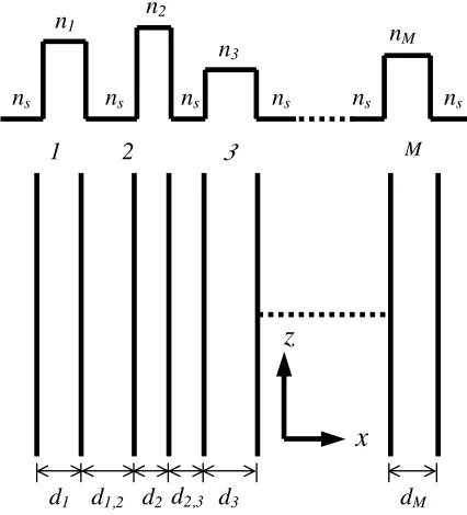
Different recurrence approaches have been used to express the dispersion relation of waveguide arrays, e.g., in [14] and [20]. The main advantage of these approaches is that they are simple to implement on computers and require fewer computational steps compared to other more complex approaches. Also, they enable monitoring the evolution of modal spectrum with each recurrence step, which not only gives an insight to the physics of modal formation in the array but also is the basis of the RZB technique proposed in this paper. In this work we follow the approach in [14] which applies for both uniform and non-uniform arrays. According to this approach the dispersion relation of an array ofM coupled waveguides (see Fig. 1) is given by,
εM = 0 (1a)
where, εM, is an implicit dispersion function of the modal effective index,N, and the free-space propagation constants,ko. It satisfies the following recurrence relation,
n1
n2
n3
nM
ns ns ns ns ns
ns
1 2 3 M
z
x
dM
d1 d1,2 d2 d2,3 d3
Figure 1. Schematic of an array of M-coupled waveguides (bottom) with the corresponding refractive index profile (top).
Here,iis the recurrence index which is incremented in steps fromi= 1 toi=M−1. The recurrence parametersJi+1 and Ki+1 are given by,
Ji+1 =Fi+1+
Ci,i+1(1−pi+1Fi+1)
2pi+Fi
1−p2i
(1−piFi)
(1c)
and
Ki+1 = Ci,i+1
1 +F2
i
(1−pi+1Fi+1)
(1−piFi)
, (1d)
with
pi =
h2i −η2iγ2
2ηiγhi
, (1e)
Ci,i+1 =
4ηiηi+1hihi+1γ2
h2
i +η2iγ2 hi2+1+η2i+1γ2
e−2γdi,i+1, (1f)
and
Fi= tan
2 tan−1(ηiγ/hi)−hidi
while the dispersion functions, ε0 = 1 and ε1 = F1. Here, hi =
ko
n2
i −N2 and γ = ko
N2−n2
s are the transverse propagation constant and the evanescent-field decay constant, respectively. The parameters,ns and ni, are the substrate refractive index and the core refractive index of the ith waveguide, respectively. The quantity, ηi, depends on the modal polarization. It equals (ni/ns)2 for TM modes and unity for TE modes. In most of photonic devices the effective indexes of the guided modes of the array satisfy the condition [14],
ns≤N ≤min
i ni. (2)
This condition means that the modal fields are oscillatory in the waveguide cores and evanescent outside these cores. As will become clear shortly, it is a key condition in simplifying the search of the roots of the dispersion equation of coupled single-mode waveguides.
3. MODIFIED DISPERSION FUNCTION
3.1. The Problem of Bracketing Singularities
Even under single-mode condition of the isolated waveguides in the array, the dispersion functionεM has singularities in the effective index,
N. As will be shown below, these singularities result from the poles of ε1, Ji+1, and Ki+1. They set up a fundamental zero-bracketing
problem [19]. For example, the opposite signs of the dispersion function between two successive values of N, may bracket a pole instead of a zero due to the discontinuity of that function. In this case, the zero search algorithm may end up returning incorrect roots of the dispersion equation. An example of such an algorithm is the built-in FZERO function in MATLAB, which is a widely used software package [21]. While, it is straightforward to discover the incorrect roots by simply evaluating the function at these roots, the absence of a clear bracketing technique implies continuing to search for the correct roots, which may potentially add to the overall computational time. Therefore, it is desirable to remove singularities of the dispersion function and to develop an efficient zero-bracketing technique to locate and compute the correct roots.
3.2. Normalization of Dispersion Function
parameters used are [22],
b = N
2−n2
s
n2
f −n2s
, (3a)
Vi = kodi
n2
f −n2s, (3b)
Vi,i+1 = kodi,i+1
n2f −n2
s. (3c)
Here,nf is the core refractive index of an arbitrarily chosen waveguide in the array. In terms of these normalized parameters the recurrence parameters,Ji+1 and Ki+1, are given by,
Ji+1=
(cot (Φi+1)−pi+1) +µi,i+1(cot (Φi) +pi)e−2Vi,i+1 √
b
(1 +pi+1cot (Φi+1))
(4a)
and
Ki+1 =µi,i+1
csc2(Φi)
(1 +picot (Φi)) (1 +pi+1cot (Φi+1))
e−2Vi,i+1√b, (4b) with
pi=
ai−
1 +ηi2 b
2ηi
b(ai−b)
, (4c)
and
µi,i+1= ηi
ηi+1
ai−b
ai+1−b ai+1+
ηi2+1−1 b ai+
η2i −1 b , (4d)
while ε0 = 1 and ε1 = cot(Φ1)−p1
1+p1cot(Φ1). Here, Φi = Vi
√
ai−b and
ai = n2
i−n2s n2
f−n2s. By combining (4) and (1b), εM becomes a function of b and the parameters, Vi, Vi,i+1, ai, and ηi. In order to identify
the singularities of εM it is required to identify the possible values that these parameters may take. Under single-mode condition of the isolated waveguides in the array, Vi√ai < π. The parameter Vi,i+1
takes any value in the range, 0< Vi,i+1 <∞. The parameter ai equals unity (for all i) in the case of uniform arrays and depends on the choice ofnf in the case of non-uniform arrays. The mode-polarization parameterηi is always greater than, or equal to, unity. The search of guided modal effective indexes satisfying condition (2) limitsbbetween 0 and 1 for uniform arrays, and between 0 and amin ≡min
3.3. Removal of Singularities from the Dispersion Function
The choice of nf = min
i ni ensures that ai ≥1 for all the waveguides in the array. In this case, b becomes limited between 0 and 1 for both uniform and non-uniform arrays. Both of these constraints on
ai and b, and the above constraint on ηi, are sufficient to eliminate any poles in pi and µi,i+1; see (4c) and (4d). Also the single-mode
condition Vi√ai < π ensures that cot (Φi) has no poles in the range, 0 < b < 1. Further inspection of ε1, Ji+1 and Ki+1 in (4), shows
that the remaining poles are only due to the zeros of (1 +picot (Φi)) and (1 +pi+1cot (Φi+1)), which appear in the denominators of these
parameters. It can be shown that neither of 1/(1 +picot (Φi)) nor 1/(1 +picot (Φi)) have zeros in the range 0< b <1, under the above constraints onVi,ai, andηi. Thus, these quantities result in redundant poles which may safely be removed without changing the zeros of the original dispersion function,εM. An induction proof for removing these poles is carried out in Appendix A. The result of removing the poles is that the dispersion equation reduces to,
χM = 0, (5a)
where the modified dispersion function, χM, satisfies the recurrence relation,
χi+1 =Di+1χi−Ei+1χi−1, (5b)
with,
Di+1 = (cot (Φi+1)−pi+1) +µi,i+1(cot (Φi) +pi)e−2Vi,i+1
√
b (5c)
and
Ei+1=µi,i+1csc2(Φi)e−2Vi,i+1 √
b. (5d)
These recurrence parameters take more simple forms compared toJi+1
and Ki+1, in (4a) and (4b). The dispersion functions, χ0 = 1 and χ1 = (cot (Φ1)−p1). Unlike εM, the modified dispersion function,
4. DIVERSITY OF DISPERSION FUNCTIONS
Thus far, the dispersion function has been modified by eliminating redundant poles from the original dispersion function. Further modification of the dispersion function may be carried out by first writing the dispersion function (5b) in terms of the determinant of a tri-diagonal matrix, as shown in Appendix B. Next by noting that
Ei+1 in (5d) does not have any zeros in the entire range, 0< b < 1,
which allows dividing the jth raw of this determinant by EM−j+1
or EM−j+1 (see Appendix B), without changing the zeros of the
dispersion function. This modification allows generating different dispersion functions which are all continuous and share the same zeros in the range, 0 < b < 1. For example, one form of the dispersion equation is given by,
δM = 0, (6a)
where the dispersion function,δM, satisfies the recurrence relation,
δi+1 =Ai+1δi−Bi+1δi−1, (6b) with the following recurrence parameters,
Ai+1=
(cot (Φi+1)−pi+1) √µi,i+1
sin (Φi)eVi,i+1 √
b
+√µi,i+1(cos (Φi)+pisin (Φi))e−Vi,i+1 √
b (6c)
and
Bi+1=
µi,i+1/µi−1,i
(sin (Φi−1)/sin (Φi))e−(Vi,i+1−Vi−1,i) √
b, (6d)
and the dispersion functions, δ0 = 1 and δ1 = {(cos(Φ1) − p1sin(Φ1))/√µ1,2}eV1,2
√
b. Indeed, δ
1, χ1, and ε1 all have the same
zeros in the range, 0 < b < 1. The particular form of the dispersion function defined by (6b)–(6d) has an advantage over other forms in the case of uniform arrays whereBi+1= 1 and,
Ai+1= (cos(Φ1)−p1sin(Φ1))eV1,2
√
b+(cos(Φ
1)+p1sin(Φ1))e−V1,2
√
b. (6e)
5. COMPUTATIONS OF THE ROOTS OF THE DISPERSION EQUATION
5.1. RZB Technique
The continuity ofδM in the range, 0< b <1, eliminates the problem of bracketing singularities in that range and allow the zeros of the dispersion function at one recurrence step to bracket its zeros at the next recurrence step. One of the primary goals of this work is to use this RZB technique to find the roots of the dispersion equation. The following numerical examples apply this technique to compute the effective indexes of the TE and TM guided modes of both uniform and non-uniform waveguide arrays.
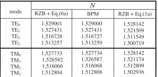
Table 1. Computed values of modal effective indexes of TE and TM modes at a freespace wavelength of λo = 1.3µm for a non-uniform array of M = 4 single-mode waveguides. The array parameters are given in the text.
1.529000 1.527431 1.516727 1.513259 TE0
TE1 TE2 TE3
1.529001 1.527431 1.516728 1.513257
1.528142 1.521509 1.511549 1.500719
N
TM0 TM1 TM2 TM3
1.527733 1.526582 1.516066 1.512804
1.528142 1.521174 1.512809 1.502936 1.527734
1.526587 1.516068 1.512808
mode RZB + Eq.(6a) BPM RZB + Eq.(1a)
5.2. Numerical Examples
5.2.1. Non-uniform Waveguide Array
This example uses a non-uniform array of M = 4 single-mode waveguides with the following design parameters. The substrate refractive index ns = 1.5. The core index of the isolated waveguides are n1 = 1.55, n2 = 1.54, n3 = 1.56, and n4 = 1.53. The
core widths are, d1 = 1.3µm, d2 = 1.1µm, d3 = 1.0µm, and d4 = 1.5, while the separation between the waveguides are, d1,2 =
2µm, d2,3 = 3µm, and d3,4 = 1µm. Table 1 shows the result of
Table 2. Computed values of modal effective indexes of TE and TM modes at a freespace wavelength of λo = 1.3µm for a uniform array of M = 8 single-mode waveguides. The array parameters are given in the text. 1.549802 1.548616 1.542330 1.532339 1.520848 1.507846 1.500872 1.500046 TM0 TM1 TM2 TM3 TM4 TM5 TM6 TM7 1.527990 1.527738 1.527337 1.526819 1.526229 1.525633 1.525111 1.524749 1.527974 1.527751 1.527345 1.526825 1.526234 1.525636 1.525111 1.524769 1.549664 1.546658 1.528778 1.525703 1.504627 1.501843 1.500448 1.500050 TE0 TE1 TE2 TE3 TE4 TE5 TE6 TE7 1.528774 1.528533 1.528151 1.527658 1.527100 1.526537 1.526047 1.525710 1.528751 1.528541 1.528154 1.527659 1.527099 1.526535 1.526041 1.525725
N
mode RZB + Eq.(6a) BPM RZB + Eq.(1a)
technique was applied with the bisection method [19] to compute the zeros of both, δM and εM, given by (6b) and (1b), respectively. The results of computations are compared with those obtained by a beam propagation method (BPM) simulator which employs an iterative technique with transparent boundary conditions [23]. The BPM computations used a computational window of 40µm, a grid size ∆x= 0.001µm, a step size in the propagation direction ∆z= 0.5µm, and an overall propagation length of 5 mm. It is shown that the RZB technique is successful in computing the zeros ofδM, and consequently the roots of the dispersion equation (6a), for both TE and TM modes. It fails to compute the roots of (1a) because of the presence of singularities in the dispersion function,εM.
5.2.2. Uniform Waveguide Array
at a free-space wavelength, λo = 1.3µm, with both the modified and conventional dispersion functions,δM and εM. In computing the zeros ofδM only one recurrence parameter was used; see (6e). The results of Table 2 show excellent agreement between the modal indexes computed using the modified dispersion function,δM, and those obtained by the iterative BPM technique. Again, the RZB technique fails in computing the zeros of εM due to the discontinuity of this function. The BPM computations used a computational window of 70µm, ∆x = 0.01µm, ∆z = 1µm, and a propagation length of 5 mm. The small difference between the modal indexes of the successive modes verify the utility of the RZB technique in resolving closely spaced roots of the dispersion equation.
6. CONCLUSION
The recurrence dispersion function of coupled waveguide arrays has been modified by removing redundant poles from this function. The removal of these poles eliminates the possibility of bracketing singularities, instead of zeros, of the modified dispersion function in the case of coupled single-mode waveguides satisfying condition (2). It has been shown that various forms of this functions may be generated which all share the same zeros. The continuity of these modified dispersion functions allows employing a simple RZB technique to locate their zeros. Numerical examples verify the utility of this technique in computing closely spaced roots of the dispersion equation.
ACKNOWLEDGMENT
This study was supported by Kuwait University research grant SP01/05.
APPENDIX A. DERIVATION OF THE MODIFIED
DISPERSION FUNCTION, χM
In this Appendix the modified dispersion function χM is derived following an induction proof. The base step is carried out by substituting with the dispersion functions ε0 = 1 and ε1 =
χ1
1
j=1
(1 +pjcot (Φj)), and the recurrence parameters, K2 and J2
of an array of two coupled waveguides,
ε2=χ2
2
j=1
(1 +pjcot (Φj)), (A1)
with χ2 = D2χ1 − E2χ0. Here, χ1 = (cot (Φ1)−p1), χ0 =
1, E2 = µ1,2csc2(Φ1)e−2V1,2
√
b, and D
2 = (cot (Φ2)−p2) + µ1,2(cot (Φ1) +p1)e−2V1,2
√ b.
In order to generalize this result for an array of M waveguides, an induction step is carried out by substituting with the dispersion
functions εM−2 = χM−2 M−2
j=1
(1 +pjcot (Φj)) and εM−1 =
χM−1 M−1
j=1
(1 +pjcot (Φj)) and the recurrence parameters Ki+1 and
Ji+1 from (4) into (1b). The results of substitution is,
εM =χM
M
j=1
(1 +pjcot (Φj)). (A2)
withχM =DMχM−1−EMχM−2 whereDM andEM are given in (5c) and (5d). Since the quantity, 1
M
j=1
(1 +pcot (Φj)), have no zeros in
the interval, 0 < b < 1, both of εM and χM share the same zeros in that interval.
APPENDIX B. MATRIX FORMULATION OF THE MODIFIED DISPERSION FUCNTION
The modified dispersion function, χM, defined by the recurrence Equation (5b) may also be defined, at each pointb, by the determinant of anM ×M tri-diagonal matrix. It can be shown using determinant properties [24] that there is no unique form of this matrix. In this Appendix we choose a symmetric form so that,χM, becomes,
χM= det
DM
√
EM 0 0 0 0 0
√
EM DM−1
EM−1 0 0 0 0
0 EM−1 DM−2
EM−2 0 0 0
0 0 • • • 0 0
0 0 0 • • • 0
0 0 0 0 √E3 D2
√ E2
0 0 0 0 0 √E2 χ1
Since Ei+1 given by (5d) is nonzero in the entire range, 0< b <1, we
can divide each raw of the above determinant byEM−j+1, wherejis
the raw index (E1 ≡E2), without changing the zeros of that function. This division results in the following from of the dispersion function,
δM = det
DM/
√
EM 1 0 0
EM/EM−1 DM−1/
EM−1 1 0
0 EM−1/EM−2 DM−2/
EM−2 1
0 0 • •
0 0 0 •
0 0 0 0
0 0 0 0
0 0 0
0 0 0
0 0 0
• 0 0
• • 0
E3/E2 D2/ √
E2 1
0 1 χ1/
√ E2
(B2)
which satisfies the recurrence relation,δi+1 =Ai+1δi−Bi+1δi−1. For
this form, the recurrence parameters,Ai+1 =Di+1 √Ei+1 andBi+1 =
Ei+1/Ei, and the dispersion functions, δ0 = 1 and δ1 = χ1 √
E2. These recurrence parameters are different fromDi+1 andEi+1 in (5c)
and (5d) due to the change in the off-diagonal matrix elements in (B2) compared to (B1). In the case of uniform waveguide arrays the lower off-diagonal elements in (B2) are all ones and the original symmetry of the matrix in (B1) is restored.
Different forms of the recurrence parameters may also be obtained following a similar approach. For each selection of these recurrence parameters the dispersion function itself changes, which verifies the diversity of the dispersion functions describing the same waveguide array. e.g., we may use the recurrence parameters,Ri+1 =Di+1/Ei+1
REFERENCES
1. Kaplan, A. and S. Ruschin, “Optical switching and power control in LiNbO3 coupled waveguide arrays,”IEEE J. Quantum Electron., Vol. 37, 1562–1573, 2001.
2. Lee, M.-H., Y. H. Min, S. Park, J. J. Ju, J. Y. Do, and S. K. Park, “Fully packages polymeric four arrayed 2 × 2 digital optical switch,”IEEE Photon. Technol. Lett., Vol. 14, 615–617, 2002. 3. Kawakita, Y., T. Saitoh, S. Shimotaya, and K. Shimomura, “A
novel straight arrayed waveguide grating with linearly varying refractive-index distribution,” IEEE Photon. Technol. Lett., Vol. 16, 144–146, 2004.
4. Kawakita, Y., S. Shimotaya, A. Kawai, D. Machida, and K. Shimomura, “Wavelength demultiplexer using GaInAs-InP MQW-based variable refractive index arrayed waveguides fabricated by selective MOVPE,” IEEE J. Select. Quantum. Electron., Vol. 11, 211–216, 2005.
5. Tangdiongga, E., Y. Liu, J. H. den Besten, M. van Geemert, T. van Dongen, J. J. M. Binsma, H. de Waardt, G. D. Khoe, M. K. Smit, and H. J. S. Dorren, “Monolithically integrated 80-Gb/s AWG-based all-optical wavelength converter,” IEEE Photon. Technol. Lett., Vol. 18, 1627–1629, 2006.
6. Choi, C.-G., S.-P. Han, B. C. Kim, S.-H. Ahn, and M.-Y. Jeong, “Fabrication of large-core 1 × 16 optical power splitters in polymers using hot-embossing process,” IEEE Photon. Technol. Lett., Vol. 15, 825–827, 2003.
7. Olivero, M. and M. Svalgaard, “Fabrication of 2 × 8 power splitters in silica-on-silicon by direct UV writing technique,”
IEEE Photon. Technol. Lett., Vol. 18, 802–804, 2006.
8. Marcuse, D.,Theory of Dielectric Optical Waveguides, Academic, New York, 1991.
9. Chilwell, J. and I. Hodgkinson, “Thin-films field transfer matrix theory of planar multiplayer waveguides and reflection from prism-loaded waveguides,”J. Opt. Soc. Am. A, Vol. 1, 742–753, 1984. 10. Walpita, L. M., “Solutions for planar optical waveguide equations
by selecting zero elements in a characteristic matrix,”J. Opt. Soc. Am. A, Vol. 2, 595–602, 1985.
11. Li, Y.-F. and J. W. Y. Lit, “General formulas for the guiding properties of a multiplayer slab waveguide,”J. Opt. Soc. Am. A, Vol. 4, 671–677, 1987.
Vol. 9, 121–129, 1992.
13. Yeh, P., “Resonant tunneling of electromagnetic radiation in superlattice structures,” J. Opt. Soc. Am. A, Vol. 2, 568–571, 1985.
14. Chiang, K. S., “Coupled-zigzag-wave theory for guided waves in slab waveguide arrays,”J. Lightwave Technol., Vol. 10, 1380–1387, 1992.
15. Anemogiannis, E. and E. N. Glytsis, “Multilayer waveguides: Efficient numerical analysis of general structures,” J. Lightwave Technol., Vol. 10, 1344–1351, 1992.
16. Smith, R. E., S. N. Houde-Walter, and G. W. Forbes, “Mode determination of planar waveguides using the four-sheeted dispersion relation,” IEEE J. Quantum. Electron., Vol. 28, 1520– 1526, 1992.
17. Chen, C., P. Berini, D. Feng, and V. P. Tozolov, “Efficient and accurate numerical analysis of multilayer planar optical waveguides,”Proc. SPIE, Vol. 3797, 676–686, July 1999.
18. Chen, C., P. Berini, D. Feng, S. Tanev, and V. P. Tozolov, “Efficient and accurate numerical analysis of multilayer planar optical waveguides,”Opt. Express, Vol. 7, 260–272, 2000.
19. Press, W. H., S. A. Teukolsky, W. T. Vetterling, and B. P. Flannery, Numerical Recipes in C: The Art of Scientific Computing, 2nd edition, Cambridge University Press, New York, 1996.
20. Ma, C., “Coupling properties in periodic waveguides and in multiple quantum-well waveguides,”IEEE J. Quantum. Electron., Vol. 30, 2811–2816, 1994.
21. The MathWorks, Inc., Natick, MA, USA.
22. Kogelnik, H., “Theory of optical waveguides,” Guided-wave Optoelectronics, T. Tamir (ed.), Ch. 2, Springer-Verlag, New York, 1990.
23. Hadley, G. R. and R. E. Smith, “Full-vector waveguide modeling using an iterative finite difference method with transparent boundary conditions,”IEEE J. Quantum. Electron., Vol. 13, 465– 469, 1995.