On the Rain-Induced Mutual Coupling Effect of Multiple-Input
Multiple-Output Communication Systems at Millimeter Wave Band
Shuhong Gong*, Xuan Wang, and Daopu Yan
Abstract—The concept of Scattering-Induced Mutual Coupling Effect (SIMCE) is proposed, and the mechanism of producing this phenomenon in Multiple-Input Multiple-Output (MIMO) communication systems at MilliMeter Wave (MMW) band is demonstrated. The model of estimating the scattering-induced mutual impedance in rain environment is derived, and the characteristics of Rain-Induced Scattering Mutual Impedance (RISMI) are discussed taking parabolic antennas as an example. The model of estimating the rain-induced mutual impedance is helpful for investigating the SIMCE in other discrete random media. And, the results given in this paper are significant for developing MMW MIMO communication systems.
1. INTRODUCTION
In comparison with traditional Single-Input Single-Output communication system, MIMO communica-tion system, which is equipped with multiple transmitting antennas and multiple receiving antennas, shows great advantages, such as higher transmission rate, better spectrum utilization ratio and greater power efficiency. Therefore, MIMO communication technology represents a breakthrough in the mod-ern communication field [1]. Many reports about MIMO communication have been focused on the frequencies below 10 GHz [1]. In recent years, some publications have paid attention to the MIMO communication at MMW band, because the communication technology at those frequencies has many advantages [1]. The study on the MIMO communication at MMW band has become a hot issue [1].
It is well known that the mutual coupling effect between antennas of a MIMO communication system impacts its performances [2–6]. But comparing with the antennas below 10 GHz, the near-field mutual coupling effect between the reflector antennas of a massive MIMO communication system at MMW band is very weak even can be neglected, because the antennas have a higher gain and a narrow beam. However, the weak near-field mutual coupling effect does not mean that the MIMO communication systems at MMW band are free from the influences of mutual coupling effect, because the so-called SIMCE exists. The SIMCE is caused by the scattering effect of the randomly distributed scatterers, such as raindrops, snowflakes and hails, in the common volume of the beams of the antennas. And, the characteristics of the SIMCE are randomly variable due to the random properties of the particles. Therefore, it is significant for developing MMW MIMO systems to investigate the properties of the SIMCE.
Without a doubt, rain-induced impacts are the first consideration aspects for designing both SISO and MIMO links working at MMW band. But the Rain-Induced Mutual Coupling Effect (RIMCE) of MMW MIMO communication systems is still in a gap status, although it really exists and is important for estimating the performances of MMW MIMO communication systems. This paper focuses on the RIMCE based on the theory of radio wave propagation and scattering in random media, antenna theory and communication fundamental. The mechanism of producing the SIMCE is analyzed. The model
Received 13 April 2015, Accepted 17 July 2015, Scheduled 9 August 2015 * Corresponding author: Shuhong Gong ([email protected]).
of estimating the RISMI is established. The characteristics of the rain-induced mutual impedance are discussed taking parabolic antennas as an example. The results given in this paper are important and helpful for developing MMW MIMO communication systems.
2. MECHANISM AND MEASUREMENT OF THE SIMCE IN MMW MIMO COMMUNICATION SYSTEMS
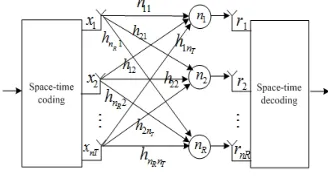
As shown in Figure 1, MIMO communication systems are equipped withnT transmitting antennas and nR receiving antennas. An overall MIMO input-output relation between the transmitting signal vector
xand the receiving signal vector yis formulated by (1) [1].
y=Hx+n (1)
where, H expresses the channel matrix, whose element hi,j (i = 1,2, . . . , mR;j = 1,2, . . . , mT) represents the random channel parameter from the jth transmitting antenna to the ith receiving antenna. nis a noise vector, the element ni is the noise into the receiver via theith receiving antenna, whose mean is 0 and variance isσ2n i.
It is well known that the mutual coupling effect between antennas of a MIMO communication system impacts its performances [2–6]. If the factor of the mutual coupling effect is taken into account, (1) should be rewritten as (2).
y=CRHCTx+n=HCx+n (2)
where, CR expresses the mutual coupling coefficient matrix of its receiving end and CT of its transmitting end. HC represents the channel matrix, in which the mutual coupling effect has been taken into account [2–6]. The mutual coupling coefficient matrix of either the transmitting end or the receiving end is closely related to its mutual impedance matrix [2–6].
Some available publications have explored several aspects of mutual coupling effect between antenna array elements on MIMO channels [7–11]. However, their research is only limited in the influences of the near-field mutual coupling effect on MIMO channels. Due to the antennas at MMW band have a higher gain and a narrower beam, once MIMO technology is applied to MMW band, the near-field-caused mutual coupling effect will decrease. Nonetheless, it does not mean that MMW MIMO systems are free from the influences of mutual coupling effect on the channel properties and the system performances, because the SIMCE exists, which is caused by the scattering effect of the randomly distributed scatterers in the common volume of the beams of the antennas, such as raindrops, snowflakes and hails. As shown in Figure 2, suppose that the transmitting antennasAandB of a MMW MIMO communication system communicate with its receiving antennas, their beams possibly intersect and form a common space. If there do not exist or exist few scatterers in the common space, the antennasAandBwill be independent of each other and will not affect each other. On the contrary, in the case where there exist a large number of scatterers, such as atmospheric turbulence, raindrops, snowflakes and hails, the electromagnetic waves radiated by the antennasAandB will be scattered in all directions by the scatterers. As a consequence, a part of radio wave transmitted by the antenna Aor the antenna B is received by the other antenna. Therefore, the SIMCE occurs. Note that although the mechanism of the occurring of the SIMCE is
explained under the assumption that the antennasAand B are in transmitting mode, the SIMCE also occurs even when they are in receiving mode [12].
Similar to the impacts of the traditional near-field mutual coupling effect on the performances of a MIMO communication system, the SIMCE also affects the performances of a MMW MIMO communication system. As a consequence, it is necessary to investigate the degree of the SIMCE for developing the MIMO technology at MMW band.
Mutual impedance or mutual coupling coefficient is often used to measure the degree of mutual coupling effect. And, as mentioned in the previous section, mutual coupling coefficient is closely related to mutual impedance. Therefore, mutual impedance is investigated to measure the degree of the SIMCE in this paper. The scattering-induced mutual impedance ZS BA of the antennaB with respect to the antennaA in Figure 2 is defined as (3) [13–15].
ZS BA=−VS BAI
A (3)
where,IAis the amplitude of an assumed current at the input port of the antennaAwhile it is assumed as in transmitting mode;VS BA denotes the open-circuited induced voltage added to the output port of the antenna B while it is assumed as in open-circuited receiving mode. Note that VS BA is induced by the scattered field ES BA, which is scattered to the antenna B by the scatterers in the common space while the radio wave radiated by the antennaAimpinges on them. In a similar manner to defineZS BA, ZS AB of the antennaA with respect to the antenna B is defined as
ZS AB =−VS ABI
B (4)
Without a doubt, rain-induced impacts are the first consideration aspects for designing both SISO and MIMO links working at MMW band. Hence, in what follows, the model of evaluating the RISMI will be established, which is used to discuss the characteristics of the rain-induced mutual impedance taking parabolic antennas as an example.
3. THE MODEL OF EVALUATING THE RISMI
In rain environment, the mutual coupling effect between antenna array elements of a MMW MIMO system is induced by the scattering of the raindrops in the common volume. In this paper, the model of evaluating the RISMI between reflector antennas is established, for reflector antennas are often used in MMW systems. While a part of the radio wave radiated by the antennaA is scattered to the reflector of the antenna B by the raindrops in the common volume, the scattered wave on the reflector will be reflected to the feed (such as a linear center-fed short dipole) of the antenna B, and ZS BA of the antennaB with respect to the antenna Ais written as
ZS-BA=−VS-BA
IA =−
l
ES BA·dl
IA =−
ES BA0·
l0
IA (5)
In Equation (5), ES-BA is the electric field vector at the point of d
l along the feed, ES-BA0 is the electric field at the center of the feed, l0 is the equivalent directed length. Note that, suppose the feed is located along a coordinate axis, usually take the positive direction of the coordinate axis as the direction of dl orl0, for convenience.
And,ES BA0 is expressed as
ES BA0 =−jωμ0 4π
s
Jτexp(jkr)
r ds (6)
In Formula (6), r is the distance from a surface elementds on the reflector to the center of the feed, ω the angular frequency, μ0 the permeability of a vacuum.
Jτ denotes the surface current density vector at the position ofds and is determined by (7) [14].
Jτ = 2ˆn×rˆ×
where, ES-R is the electric field vector of the scattered wave at the position of ds, ˆn the normal unit vector at the position ofds, and ˆr the unit vector of the propagation direction of the scattered wave. η represents the wave impedance of rain environment and can be estimated by
η=
εeff μ0
(8)
where, εeff is the equivalent permittivity of rain environment [16].
ES-R in Equation (7) can be calculated by
ES-R= Dmax
Dmin
VC
ES(D)N(D)dV dD (9)
In Equation (9), VC denotes the volume of the common space, D the diameter of a raindrop in VC, N(D) the raindrops size distribution function,ES(D) the scattered field by a raindrop with a diameter D, andDminandDmaxare respectively the minimum and the maximum ofD.
ES(D) can be calculated with a good approximation by Mie theory [17]. The components of ES(D) in the θ-direction and the ϕ-direction in Figure 3 are written as (10) and (11) [17].
ES θ(D) =EAexp(−γ1−γ2)iS2 (D, θs)
krs exp(ikrs) cosϕs (10)
ES ϕ(D) =−EAexp(−γ1−γ2)iS1 (D, θs)
krs exp(ikrs) sinϕs (11) where,rsis the distance from the raindrop to the position ofdson the reflector; EAis the amplitude of the electric field at the raindrop’s position radiated by the antennaA;γ1andγ2 are the path attenuation of the incident wave and the scattered wave, respectively; S1(D, θs) and S2(D, θs) are the scattering amplitude functions which are elaborated in [17]; θs and ϕs are the scattering angle and the scattering azimuth angle in Figure 3, respectively.
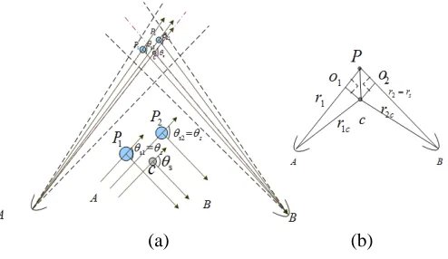
As the antennas at MMW band have a very high gain and very narrow beam, it is logical and convenient to make the following approximate assumptions: the scattering angles of any two raindrops in the common space, such as the scattering angles of the two raindrops at P1 and P2 in Figure 4(a), are identical and equal the scattering angle of the raindrop at the center of the common space, namely at the intersection c of the central axes of the two beams in Figure 4(a) and Figure 4(b); the incident wave on the common space has a plane wave-front, on which the electric field has the same amplitude of 0.8535EA, see Figure 4(a), whereEAis the amplitude of the electric field at the intersection between
Figure 3. The sketch of Mie scattering of a raindrop.
(a) (b)
the wave-front and the beam central axis of the antennaA; the distances associated with the amplitude and the attenuation in (10) and (11), such as rs in the dominator of Equations (10) and (11),r1 andr2 for calculating the attenuation γ1 and γ2 in Equations (10) and (11), can be replaced by the distance to the intersection c, but the distance for estimating the phase factor in Equations (10) and (11) need to use the real distance r1 and r2, see Figure 4(b). Note that 0.8535 = (1 + 0.707)/2, that is, suppose it is approximately true that the magnitude of the electric field linearly reduced from the center of the beam to the position of the half-power beam width. The approximation is logical for an antenna whose half-power beam width is less than 10◦.
According to the approximate assumptions mentioned above, the components of ES-R in the θ -direction and theϕ-direction can be derived as
ES-R-θs = Dmax
Dmin
0.8535EAexp(−γ1c−γ2c)iS2
(D, θsc) kr2c
exp(ikr2c)
·cosϕscN(D)
VC
exp [ik(P o1+P o2)]dV dD (12)
ES-R-ϕs = Dmax
Dmin
−0.8535EAexp(−γ1c−γ2c)iS2
(D, θsc) kr2c
exp(ikr2c)
·sinϕscN(D)
VC
exp [ik(P o1+P o2)]dV dD (13)
where, θsc and ϕsc are the scattering angle and the scattering azimuth angle of the raindrop at the intersection c, respectively; P o1 and P o2, r1c and r2c are shown in Figure 4(b); γ1c and γ2c can be approximately estimated by (14).
γ1c=γ·r1c·10−3/8.686 γ2c=γ·r2c·10−3/8.686
(14)
where, γ represents the specific attenuation in rain environment, which is elaborated in [18].
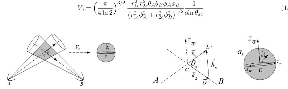
As shown in Figure 5, the common space is an irregular volume, so it is difficult to calculate the integrals in (12) and (13). Therefore, it is necessary to make an equivalent approximation for the common space. In this paper, the irregular common space is simplified as a sphere with the same volume as that of the irregular common space. The center of the equivalent sphere overlaps the center cof the common space.
For the narrow beam antennas, the volume of the common space of the two beams can be approximately estimated by [17]
Vc =
π
4 ln 2
3/2 r2
1cr22cθAθBφAφB
r2
1cφ2A+r22cφ2B
1/2 1
sinθsc (15)
Figure 5. The schematic of the irregular volume and the equivalent sphere.
where, θA,θB andφA,φB represent the half power beam width of the vertical plane and the horizontal plane of the antennasA and B. As a consequence, the radius of the equivalent sphere can be given as
as= 1024(ln 2)9π 3
1/6
r21cr22cθAθBφAφB
r12cφ2A+r22cφ2B
1/2 1 sinθsc
1/3
(16)
For convenience’s sake, as shown in Figure 6, select the direction of the vectorks=
k1−
k2 as the Zsp-axis ofXsp-Ysp-Zsp, which is the local spherical coordinate system to describedV in Equations (12) and (13). As a consequence,k(P o1+P o2) in Equations (12) and (13) can be approximately expressed as (17).
k(P o1+P o2) = 2ksin
θsc 2
cos(θ) (17)
where, θ is shown in Figure 6. Therefore, the volume integral in Equations (12) and (13) can be presented as
int =
V e
ik(P o1+P o2)dV =
2π 0 dϕ π 0 sinθdθ as 0
ei2 sin(θsc/2)krcosθr2dr
= 4π
[2 sin(θsc/2)k]{[2 sin(θsc/2)kas] cos [2 sin(θsc/2)kas]−sin [2 sin(θsc/2)kas]} (18)
Note that it is necessary to convert the results in (12) and (13) into the components ofES-Rin the coordinate system for depicting the function of the curved surface of the antennaB, because the results in Equations (12) and (13) are given in the spherical coordinate system in Figure 3. In addition, the magnitude of the electric field at the vertex of the reflecting surface of the antennaB can be expressed as the results in Equations (12) and (13), however, that at any point should be given as
ES-R-θs = Dmax
Dmin
0.8535EAexp(−γ1c−γ2c)iS2
(D, θsc) kr2c ·
exp[ik(r2c −Δr] cosϕscN(D)(int)dD (19)
ES-R-ϕs = Dmax
Dmin
−0.8535EAexp(−γ1c−γ2c)iS
2(D, θsc) kr2c ·
exp[ik(r2c−Δr)] sinϕscN(D)(int)dD (20)
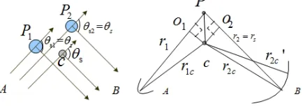
where, Δr=r2c−r2c denotes a distance difference betweenr2c and r2c as shown in Figure 7.
Figure 7. The sketch for interpreting Δr in Equations (19) and (20).
In a similar manner to deriving the model for calculating ZS BA in rain environment, the model for calculating ZS AB in rain environment can be derived. It is reasonable to consider that ZS BA approximatively equals ZS AB in rain environment, because Mie theory [17] can be used for calculating the scattered field of the raindrops with a good approximation.
4. THE SIMULATION RESULTS OF THE SCATTERING MUTUAL IMPEDANCE BETWEEN TWO PARABOLIC ANTENNAS
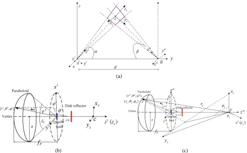
As shown in Figure 8, suppose that the same two front-fed rotating parabolic antennas, whose feeds are a linear center-fed short dipole with a dish reflector, are adopted in a MMW MIMO system. For convenience and without loss of generality,ZS BAis calculated by using (5) under the assumptions that the antenna A in Figure 8 is in transmitting mode and the antenna B is in open-circuited receiving mode.
In Figure 8, α and β denote the elevation angles of the antennas A and B respectively; d is the distance between the antennasA and B;c is the center of the common volume; the coordinate system x-y-zis used to determine the relative location of the antennas AandB; the coordinate systemx-y-z is used to describe the antenna A and x-y-z the antenna B; the coordinate system xs-ys-zs is used to present the scattered field of the raindrops in the common volume; a represents the radius of the aperture plane of the antennasAand B;fp denotes the focal length; ˆnis the unit vector of the normal direction of any point on the paraboloid; ξ0 is the aperture angle of the antennas; x-y-z is obtained by clockwise rotating x-y-z an angle 90-α around itsx axis; xs-ys-zs is obtained by translating x-y-z along thez axis;x-y-z is got by firstly anticlockwise rotatingx-y-zan angel 90-β around itsxaxis, then translating the rotated coordinate a distancedalong the positive direction of the y axis of x-y-z. Note that during the simulation it is necessary to relate the space variables in one of these rectangular coordinate systems such as (x, y, z) to those in the spherical coordinate system defined by itself such as (r, θ, ϕ), to relate the space variables in one of these coordinate systems such as (xs, ys, zs) to those in another different coordinate system such as (x, y, z). The coordinate transformation matrix, which relates coordinates and basis vectors in one frame to those in another frame, can be found in some relevant publications such as [19, 20].
Based on Figure 8, the necessary parameters for simulating the rain-induced mutual impedance can be obtained. For example, θsc = 180−α−β; r1c and r2c can be given by solving the following
(a)
(b) (c)
equation set
r1c·cosα+r2c·cosβ=d r1c·sinα=r2c·sinβ
(21)
ϕsc can be obtained by transforming the components (r, θ, ϕ) of the vector OQ in x-y-z into the components (rs, θs, ϕs) of the vector cQ in xs−ys−zs; Δr =rs−r2c−fp.
According to the publication of [14], the radiated electric-field of the antennaAin Figure 8 is linear polarization along thex-axis, andEA at pointc is derived as
EA= 120π 2I
Al0a2 λ2r
1cfP
1.48J1(7a/4fp)J0(0) (7a/4fp) −
3J2(0)J1(21a/8fp) (21a/8fp)2
(22)
And, for the antennas in Figure 8, the half power beam width of E-plane or H-plane in (15) and (16) is related to a/2fp. During the simulation in this paper, suppose that the half power beam width of E-plane is 3◦ and a/2fp = 0.4, which means that θA=θB = 3◦ and ϕA=ϕB = 2.9◦ in (15) and (16), a= 63λ/6, fp=a/0.8 [14].
At the position of a surface element ds on antenna B, the total scattered electric-field by the raindrops in the common volume can be calculated by substituting (22) into (19) and (20). Relate the electric-field components ofES-R-θs andES-R-ϕs inxs-ys-zs to those ofES-R-x,ES-R-y andES-R-z in
Figure 9. The changing relationship of ZS BA with R under the conditions of the same d, α, β and the different f.
Figure 10. The changing relationship of ZS BA withR under the conditions of the samed,f and the different α,β.
Figure 12. The changing relationship of ZS BA with dunder the conditions of the same α, β,f and the different R.
Figure 13. The changing relationship ofZS BA withdunder the conditions of the sameR,f and the different α,β.
x-y-z, also relate the components of the unit vector ˆr of the scattered wave propagation direction in xs-ys-zs to those in x-y-z, then the components of the vector of the surface current density at the position of ds can be obtained by using (7). The rain-induced mutual impedance of the two antennas in Figure 8 can be estimated by using (5). In this simulation example, the Weibull raindrops size distribution function [21, 22] is employed as N(D).
For the two antennas in Figure 8, Figure 9–Figure 11 show the changing relationship of their rain-induced mutual impedance with rain rate R when the parameters of d, α, f are specified, Figure 12– Figure 14 with the distancedbetween the two antennas when the parameters ofR,α,β f are specified, and Figure 15–Figure 17 with frequency f when the parameters of d, α, β R are specified. In what follows, the simulation results are listed and discussed.
Figure 9–Figure 11 show that the changing trend of the RIMCE with rain rate increase is related with the other parameters such asα,β,dandf. Figure 9 displays that for the sameα,βand d,ZS BA increases more slowly at 50 GHz than at 35 GHz with rain rate increase, because the rain-induced attenuation at 50 GHz is severer than that at 35 GHz, as well as because the scattering properties of raindrops are different at the two frequencies. In fact, it can be concluded that due to the severer attenuation at higher frequencies,ZS BAmaybe firstly increase and then decrease withRincrease, which is jointly determined by the attenuation and the scattering properties at those frequencies. Figure 10 and Figure 11 imply that α, β and d can impact the trend of ZS BA varying with R by changing the size of the common volume and the severity degree of the attenuation. The larger common volume and the less attenuation will enhance the RIMCE, whereas the RIMCE will be reduced.
Figure 15. The changing relationship ofZS BA with frequency under the conditions of the samed,R and the different α,β.
Figure 17. The changing relationship of ZS BA with f under the conditions of the same R,α,β and the different d.
Figure 12–Figure 14 display thatZS BA presents an oscillation variation trend with the change of d, what is more, f,α and β obviously alter the oscillation period. In addition, as mentioned above, the scattering properties of the raindrops, the severity degree of the attenuation and the size of the common volume jointly determineZS BA, therefore the envelops in Figure 12–Figure 14 firstly increase and then decrease with dincrease.
Similar to the variation relationship of ZS BA with d, ZS BA in Figure 15–Figure 17 vary in fluctuation with f. And d, α, β are sensitive to the fluctuation period. For the same reasons stated above, the envelops in Figure 15–Figure 17 also firstly increase and then decrease with f increase.
5. CONCLUSIONS
This paper focuses on the RIMCE of MMW MIMO communication systems. The conclusions from the simulation results in this paper are summarized in what follows:
The simulation results in this paper signify that ZS BA is about in the dozens to hundreds of Omegas magnitude, which means thatZS BA cannot be ignored. In other words, the RIMCE is a new necessary consideration aspect for developing MMW MIMO communication technology.
The characteristics of the oscillation variations of ZS BA with d and f, of the dependence relationship of the oscillation periods on d,f,α andβ, imply that it is feasible to reduce the negative impact of the RIMCE on MMW MIMO communication systems by optimizing their link parameters. That is, the model for estimating rain-induced mutual impedance derived in this paper is significant for designing a MMW MIMO link.
Therefore, it can be concluded from this paper that the RIMCE is a new necessary consideration aspect for developing MMW MIMO communication systems and that the model for estimating rain-induced mutual impedance derived in this paper is significant for designing a MMW MIMO link.
ACKNOWLEDGMENT
The authors would like to thank the National Natural Science Foundation of China under Grant No. 61001065.
REFERENCES
1. Gong, S. H., D. X. Wei, X. W. Xue, and M. Y. H. Chen, “Study on the channel model and BER performance of single-polarization satellite-earth MIMO communication systems at Ka band,”
2. Svantesson, T. and A. Ranheim, “Mutual coupling effects on the capacity of multi-element antenna systems,”Proc. IEEE ICASSP 2001, 2485–2488, Salt Lake City, UT, 2001.
3. McNamara, D. P., M. A. Beach, and P. N. Fletcher, “Experimental investigation into the impact of mutual coupling on MIMO communications systems,”Proc. of Int. Symp. on Wireless Personal Multimedia Communications, Vol. 1, No. 9, 169–173, 2001.
4. Fletcher, P. N., M. Dean, and A. R. Nix, “Mutual coupling in multi-element array antennas and its influence on MIMO channel capacity,” Electron. Lett., Vol. 39, No. 4, 342–342, 2003.
5. Clerckx, B., D. Vanhoenacker-Janvier, C. Oestges, and L. Vandendorpe, “Mutual coupling effects on the channel capacity and the space-time processing of MIMO communication systems,” IEEE Int. Conf. Communication’03, 2638–2642, 2003.
6. Ji, L., “Studies on modeling and simulation of multiple-input multiple-output wireless channel and analysis of channel properties with mutual coupling,” Ph.D. Dissertation, Department National University of Defense Technology, Changsha, China, 2006.
7. Fang, Y., “Array antenna mutual coupling analysis,” Hans Journal of Wireless Communications, Vol. 3, No. 1, 1–13, 2013.
8. Cheng, Y., R. Yu, H. Gu, et al., “Multi-SVD based subspace estimation to improve angle estimation accuracy in bistatic MIMO radar,” Signal Processing, Vol. 93, No. 7, 2003–2009, 2013.
9. Yun, J. X. and R. G. Vaughan, “Evaluating multi-element antennas using equivalent number of antenna elements,”IEEE 2013 7th European Conference on Antennas and Propagation (EuCAP), 89–32, 2013.
10. Dehghani, E. M. and R. G. Vaughan, “On the power delay profile and delay spread for the physics-based simulated mobile channel,” IEEE 2013 7th European Conference on Antennas and Propagation (EuCAP), 959–963, 2013.
11. Sanchez-Hernandez, D., M. Rumney, R. J. Pirkl, and M. H. Landmann, “MIMO over-the-air research, development and testing,” International Journal of Antennas & Propagation, Vol. 6, No. 3, 601–617, 2012.
12. Balanis, C. A., Antenna Theory: Analysis and Design, 3rd Edition, Wiley-Interscience, Hoboken, 2005.
13. Xue, C. F. and W. J. Qiu,Antenna Theory and Design, Northwest Telecommunication Engineering Institute Press, Xi’an, 1985.
14. Wei, W. Y. and D. M. Gong, Antenna Theory, National Defense Industry Press, Beijing, 1985. 15. Thomas, A. M., Modern Antenna Design, 2nd Edition, Wiley-Interscience, Hoboken, 2005.
16. Gong, S. H. and J. Y. Huang, “Accurate analytical model of equivalent dielectric constant for rain medium,”Journal of Electromagnetic Waves and Applications, Vol. 20, No. 13, 1775–1783, 2012. 17. Ishimaru, A., Wave Propagation and Scattering in Random Media, IEEE Press, New York, 1978. 18. Gong, S. H., “Study on some problems for radio wave propagating and scattering through
troposphere,” Ph.D. Dissertation, Department Science, Xidian University, Xi’an, China, 2008. 19. Spigel, M. R., J. Liu, and G. J. Hademenos, Mathematical Handbook of Formulas and Tables,
McGraw-Hill, New York, 1968.
20. Grewal, M. S., L. R. Weill, and A. P. Andrews, Global Positioning System, Inertial Navigation, and Integration, John Wiley & Sons, Hoboken, 2001.
21. Marshall, J. S. and W. M. Palmer, “The distribution of raindrops with size,”Meteor, Vol. 5, No. 4, 165–166, 1948.